March 28, 2023 26 min to read

StatsBomb Data Exploration pt1

Introduction to exploring football data with StatsBomb

Exploring StatsBomb Python API and Datasets for Football Analysis and Visuals

Code and notebook for this post can be found here.

This post is part of a series focusing on the exploration of StatsBomb’s Python API and datasets for football analysis and creating visuals. We will utilize web-scraping techniques to extract relevant football data and leverage the available Python packages to conduct an analysis.

The primary aim of this project is to harness the power of python coding and StatsBomb’s data to achieve the following objectives:

• Develop efficient functions to aggregate data from StatsBomb python API.
• Perform data manipulation tasks to transform raw data into clean, structured datasets suitable for analysis.
• Create visually appealing data visualizations using the obtained datasets.
• Evaluate significant metrics that aid in making assertions on players & team performance.

By accomplishing these objectives, we will gain valuable insights into football analysis and visualization techniques. This project serves as a foundation for further exploration of StatsBomb’s Python API and datasets, offering opportunities to expand the scope of analysis and delve deeper into football analytics.

The code and examples provided in the notebook showcase the potential of utilizing StatsBomb’s data for football-related projects.

Setup

We will need to import several Python libraries that will be key in our tasks.

We start by importing statsbombpy, which is a Python package that provides convenient access to the StatsBomb API. This API allows us to retrieve comprehensive football data, including information about competitions, matches, players, and more. The followinggithub-repo goes in to great depths as to how the package works and how you can find the tables you need.

from statsbombpy import sb
import pandas as pd
from pandas import json_normalize
import numpy as np

import matplotlib.pyplot as plt
import matplotlib.ticker as ticker
import matplotlib.patheffects as path_effects

# We'll only use a vertical pitch for this tutorial
from mplsoccer import VerticalPitch, Sbopen

# Get competitions
comp = sb.competitions()
comp.to_csv('competitions.csv', index=False)

To create visualizations, we utilize the matplotlib library, which provides a flexible and powerful framework for generating various types of plots and charts. We also import matplotlib.ticker to customize the tick placement on our plots and matplotlib.patheffects to add special effects to our plot elements.

Additionally, we import the VerticalPitch class and Sbopen function from mplsoccer. These components are part of the mplsoccer package, which specializes in creating football visualizations. In our case, we will focus on utilizing the vertical pitch functionality to construct insightful and visually appealing football graphics.

Finally, we initiate our data exploration by obtaining information about competitions using the sb.competitions() function. This function retrieves the available competitions from the StatsBomb API and stores the data in a CSV file named competitions.csv.

We will also need to install other necessary packages such as mplsoccer. This package provides us with powerful tools for creating football visualizations. You can install it using the following command:

pip install mplsoccer

Exploratory Data Analysis

Now that all our packages are installed, we can start looking at the data. The code provided below demonstrates the use of the statsbombpy library to retrieve and save match data from the 2022 FIFA World Cup. For this post we will be using England’s quarter final win over Senegal as the match we’ll look at.

First, we retrieve the matches from the World Cup using the sb.matches() function from statsbombpy. We specify the competition ID as 43 (which corresponds to the FIFA World Cup) and the season ID as 106 (which represents the 2022 season). The resulting matches are stored in a DataFrame called df, and then saved as a CSV file named ‘WC_Matches.csv’ using the to_csv() method.

# Get Matches from 2022 FIFA World Cup
df = sb.matches(competition_id=43, season_id=106)
df.to_csv('CSVs/WC_Matches.csv', index=False)

Next, we identify a specific match using its match ID. In this case, the match ID is 3869118. We pass this ID to the sb.events() function from statsbombpy to retrieve the events data for that particular match. The events data is stored in a DataFrame called match_events.

Finally, we extract the unique team names from the team column of match_events and store them in a list called team_list . These team names represent the teams involved in the match.

Overall, this code fetches match data from the 2022 FIFA World Cup, saves it to a CSV file, and extracts the team names for further analysis or visualization purposes.

# Find a match_id required for England vs Sengal
match = 3869118
match_events = sb.events(match_id=match)
team_list =list(match_events.team.unique())

Dataframe Manipulation

In this code block, we are processing the match_events DataFrame to extract pass-related data for the first half of the match.

• We first create a new DataFrame called first_half by filtering match_events to include only rows where the ‘period’ column is equal to 1, representing the first half of the match.

• Similarly, we create a DataFrame called second_half by filtering match_events to include only rows where the ‘period’ column is equal to 2, representing the second half of the match.

• Next, we filter the first_half DataFrame further to include only rows where the ‘type’ column is equal to ‘Pass’, resulting in a DataFrame called pass_raw.

• Finally, we select specific columns ('timestamp', 'player', 'pass_recipient') from pass_raw and store the result in the pass_number_raw DataFrame.

first_half = match_events.loc[match_events['period'] == 1] 
second_half = match_events.loc[match_events['period'] == 2] 

pass_raw = first_half[match_events.type== 'Pass']

pass_number_raw = pass_raw[['timestamp', 'player', 'pass_recipient']]

pass_number_raw DataFrame, representing the pairing of players involved in each pass.

We create a new column called ‘pair’ in the pass_number_raw DataFrame by concatenating the ‘player’ and ‘pass_recipient’ columns using the ‘+’ operator.

The resulting ‘pair’ column contains the combined names of the player and pass recipient for each pass.

Dataframe Calculations

pass_number_raw['pair'] = pass_number_raw.player + pass_number_raw.pass_recipient

In this code block, we are calculating the number of passes between player pairs using the pass_number_raw DataFrame.

We group the pass_number_raw DataFrame by the ‘pair’ column, which represents the player pairs, using the groupby() function.

We then apply the count() function to count the number of occurrences for each unique player pair. The resulting DataFrame is stored in the pass_count variable, including the ‘pair’ column and a new column ‘timestamp’ that contains the count of passes.

Finally, we update the column names to ‘pair’ and ‘number_pass’ using the columns attribute.

pass_count = pass_number_raw.groupby(['pair']).count().reset_index()
pass_count = pass_count[['pair', 'timestamp']]
pass_count.columns = ['pair', 'number_pass']
pass_count.head()

Now, for the purposes of keeping this interesting, lets start to make some nice pictures.

Building Visualisations

Team Pass Maps

In order to efficient create basis for the data that will feed our visuals, lets create some functions that will tick off our initial objective of Develop efficient functions to aggregate data from StatsBomb python API.

The function create_passmap_df() takes in two arguments: a string representing a national team and a pandas DataFrame with match events. It returns another DataFrame with pass data.

The code separates the first and second halves, extracts pass events from the first half, and obtains relevant columns. It calculates pass counts between player pairs and average player locations.

The resulting data is merged and cleaned.

It creates player statistics and selects top players. Passes between them are filtered and width is calculated. Finally, the code returns the filtered pass data with added width column.

Functions

def create_passmap_df(national_team:str,match_events:pd.DataFrame):
    
    first_half = match_events.loc[match_events['period'] == 1] 
    second_half = match_events.loc[match_events['period'] == 2]
    pass_raw = first_half[match_events.type== 'Pass']
    pass_number_raw = pass_raw[['timestamp', 'player', 'pass_recipient']]
    pass_number_raw['pair'] = pass_number_raw.player + pass_number_raw.pass_recipient
    pass_count = pass_number_raw.groupby(['pair']).count().reset_index()
    pass_count = pass_count[['pair', 'timestamp']]
    pass_count.columns = ['pair', 'number_pass']

    avg_loc_df = pass_raw[['team', 'player', 'location']]
    avg_loc_df['pos_x'] = avg_loc_df.location.apply(lambda x: x[0])
    avg_loc_df['pos_y'] = avg_loc_df.location.apply(lambda x: x[1])
    avg_loc_df = avg_loc_df.drop('location', axis=1)

    avg_loc_df = avg_loc_df.groupby(['team','player']).agg({'pos_x': np.mean, 'pos_y': np.mean}).reset_index()

    pass_merge = pass_number_raw.merge(pass_count, on='pair')
    pass_merge = pass_merge[['player', 'pass_recipient', 'number_pass']]
    pass_merge = pass_merge.drop_duplicates()

    avg_loc_df = avg_loc_df[['player', 'pos_x', 'pos_y']]

    pass_cleaned = pass_merge.merge(avg_loc_df, on='player')
    pass_cleaned.rename({'pos_x': 'pos_x_start', 'pos_y': 'pos_y_start'}, axis='columns', inplace=True)

    pass_cleaned = pass_cleaned.merge(avg_loc_df, left_on='pass_recipient', right_on='player', suffixes=['', '_end'])
    pass_cleaned.rename({'pos_x': 'pos_x_end', 'pos_y': 'pos_y_end'}, axis='columns', inplace=True)

    # pass_cleaned = pass_cleaned.drop(['player_name_end'], axis=1)

    player_df = first_half[first_half.team == national_team ].groupby('player').agg({'minute': [min, max]}).reset_index()
    player_df = pd.concat([player_df['player'], player_df['minute']], axis=1)
    player_df['minutes_played'] = player_df['max'] - player_df['min']
    player_df = player_df.sort_values('minutes_played', ascending=False)

    player_names = player_df.player[:11].tolist()

    pass_team = pass_cleaned[pass_cleaned.player.isin(player_names)]
    pass_team = pass_team[pass_team.pass_recipient.isin(player_names)]

    pass_team['width'] = pass_team['number_pass'] / pass_team['number_pass'].max()

    return pass_team

pass_df = create_passmap_df("England",match_events)

The resulting dataframe for england is showin the table below:

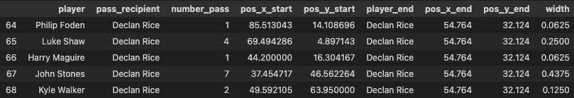
Now that we have our dataframe ready, we can use that to build our first visual.

The following code creates a football pitch using the VerticalPitch function from the mplsoccer library. The pitch is set to use the StatsBomb pitch type, which is a specific format for the data we will pass in.

After that, the code creates the plot and sets the size and position of the pitch on the plot. The plot includes the passing lines and nodes, which will show the passing patterns of the team.

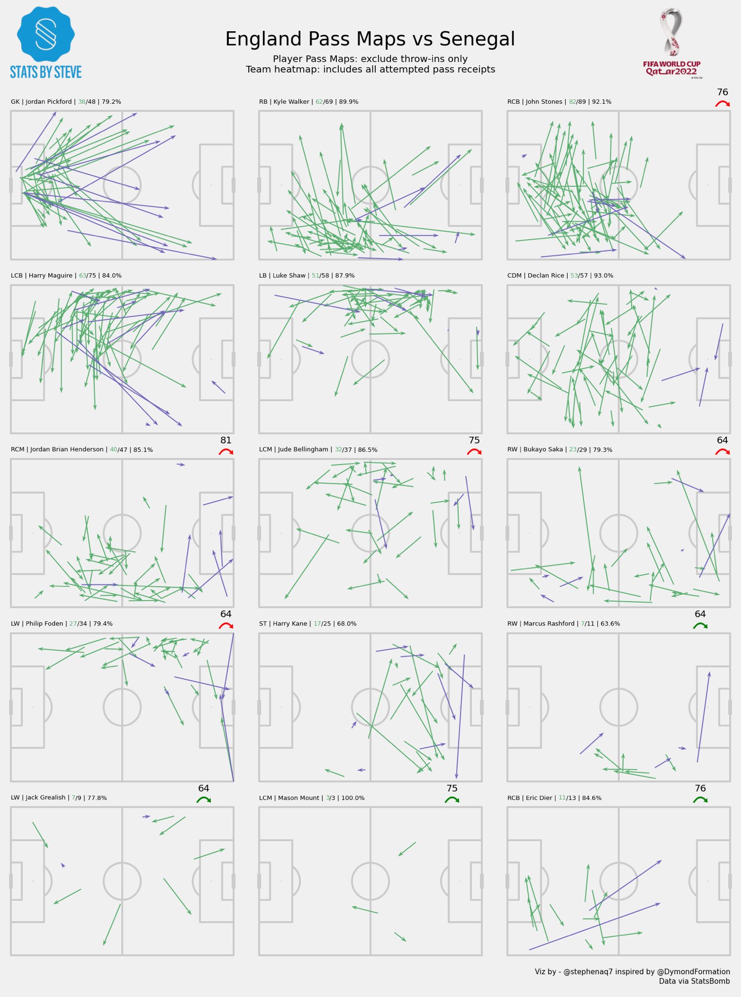
The code then adds annotations to the plot, indicating the players who made the passes. It also adds logos for the FIFA World Cup and the creator of the plot.

Finally, the code adds a title to the plot that displays the names of the two teams playing and which half of the match the plot is showing. The plot is then saved and displayed.

from matplotlib.colors import to_rgba
import matplotlib.style as style
from PIL import Image
import matplotlib.image as image


style.use('fivethirtyeight')

MIN_TRANSPARENCY = 0.1
color = np.array(to_rgba('black'))
color = np.tile(color, (len(pass_df), 1))
c_transparency = pass_df.number_pass / pass_df.number_pass.max()
c_transparency = (c_transparency * (1 - MIN_TRANSPARENCY)) + MIN_TRANSPARENCY
color[:, 3] = c_transparency

pitch = VerticalPitch(pitch_type='statsbomb', 
    half = False,
    axis = True, 
    # label = True, 
    # tick = True,
    goal_type='box')
    
fig, axs = pitch.grid(figheight=10, title_height=0.08, endnote_space=0, axis=False, 
                      title_space=0, grid_height=0.82, endnote_height=0.05)


pass_lines = pitch.lines(pass_df.pos_x_start, pass_df.pos_y_start,
                         pass_df.pos_x_end, pass_df.pos_y_end, 
                         lw=pass_df.width+0.5,
                         color=color, zorder=1, ax=axs['pitch'])

pass_nodes = pitch.scatter(pass_df.pos_x_start, pass_df.pos_y_start, s=350,
                           color= '#a71c1c', linewidth=1, alpha=0.1, ax=axs['pitch'])

for index, row in pass_df.iterrows():
    pitch.annotate(row.player, xy=(row.pos_x_start-3, row.pos_y_start-3), c='#0b5394', va='center',
                   ha='center', size='small', weight = 'light', family='sans-serif', ax=axs['pitch'],stretch= 'ultra-condensed',style="normal" ,alpha=0.5)
    
# endnote /title
axs['endnote'].text(1, 0.5, '@stephenaq7',
                    va='center', ha='right', fontsize=10)
axs['endnote'].text(1, 0.1, 'data via StatsBomb',
                    va='center', ha='right', fontsize=8)

### Add Fifa WC logo
ax2 = fig.add_axes([0.8, 0.035, 0.175, 1.8])
ax2.axis('off')
img = image.imread('/Users/stephenahiabah/code/statsbomb_project/FWC_Logo.png')
ax2.imshow(img)


### Add Stats by Steve logo
ax3 = fig.add_axes([0.008, -0.028, 0.17, 0.15])
ax3.axis('off')
img = image.imread('/Users/stephenahiabah/code/statsbomb_project/logo_transparent_background.png')
ax3.imshow(img)

axs['title'].text(0.4, 1, f'FWC 2022 - {team_list[0]} vs {team_list[1]} ', weight = 'bold', alpha = .75,
                  va='center', ha='center', fontsize=18)
axs['title'].text(0.25, 0.25, f'{team_list[0]}  - 1st Half Passing Network',
                  va='center', ha='center', alpha = .75, fontsize=12)
plt.savefig(f'Output Visuals/{team_list[0]} - Passing Networks.png', dpi=300, bbox_inches='tight')
plt.show()

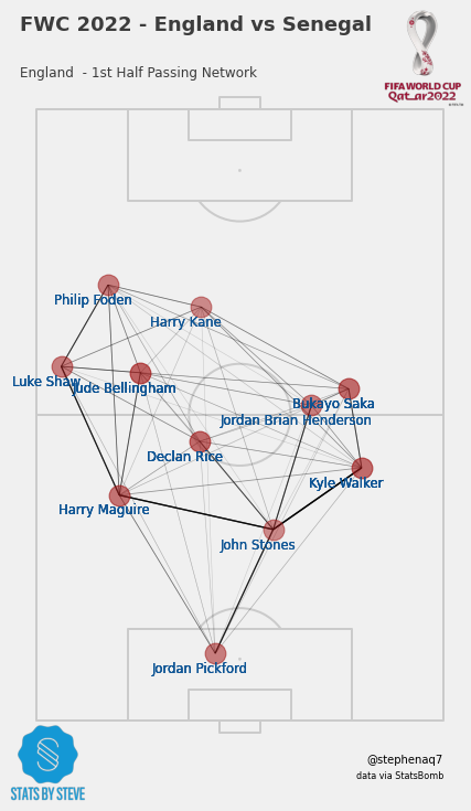
Overall, the code creates a passing network visualization for a football match, showing the passing patterns of a team during a certain half of the match. The visualization is complete with annotations and logos to make it look professional.

Shot Maps

Now that we’ve done passing, naturally lets move on to shots and xg etc.

By changing the the match_events column varianle to ‘shot’, we can create a new dataframe with shot & their location.

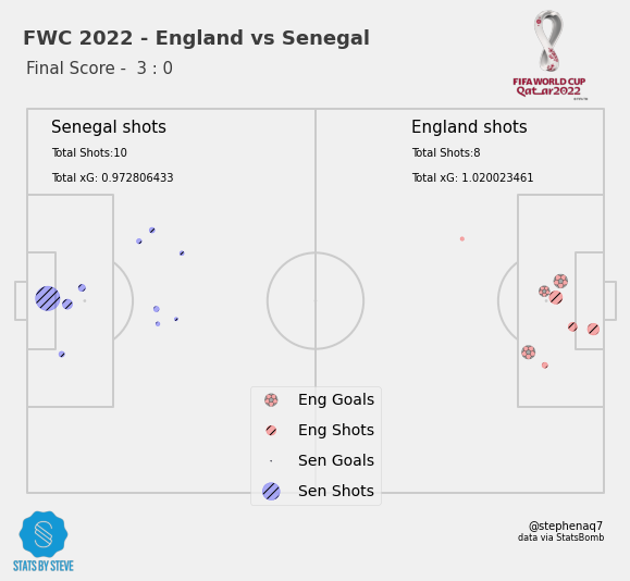
Let’s create a clean shots dataset with shot locations to create a shot xg map like this

shot_raw = match_events[match_events.type== 'Shot']
shot_raw["location"] = shot_raw["location"].astype(str)
shot_raw["location"] = shot_raw["location"].str[1:]
shot_raw["location"] = shot_raw["location"].str[:-1]
shot_raw[["location"]]
shot_raw[["x", "y"]] = shot_raw["location"].str.split(",", expand=True).astype(np.float32)

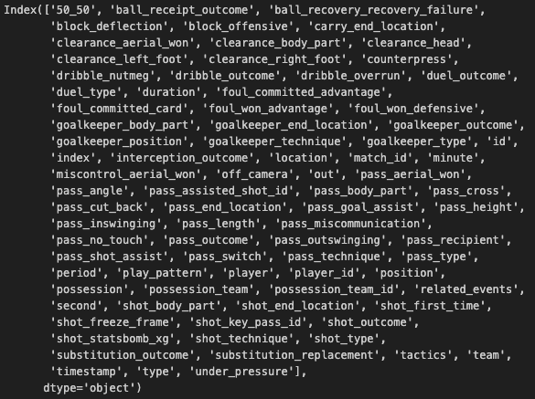
The code filters the match events dataframe to only include events of type “Shot” and assigns it to the variable shot_raw. It then performs some data cleaning on the “location” column within shot_raw.

First, it converts the “location” column to a string type. Then, it removes the first and last characters of each string value, effectively removing the brackets around the coordinates.

Next, it splits the cleaned “location” strings by the comma separator and expands them into separate columns “x” and “y”.

Finally, it converts the values in these columns to floating-point numbers using the NumPy library’s astype(np.float32) function. The resulting dataframe shot_raw now contains the cleaned “x” and “y” coordinates of the shot locations.

Here is a view of the columns in the resulting shot_raw df:

First, we imports two libraries: Seaborn and Mplsoccer. Then, there are two functions defined in the code. The first function is called generateTeamxGDataFrame() and it takes one argument, which is the name of a team. The function generates a dataframe containing data on the team’s shots during the match, including information like the time the shot was taken, the position on the field, and the expected goal (xG) value of each shot.

The second function is called generateCombinedShotMap() and takes two arguments, which are the names of the two teams in the match. This function uses the generateTeamxGDataFrame() function to generate dataframes for each team’s shots. Then, it uses the Mplsoccer library to create a visualization of the shots on the soccer field, with different colors and symbols representing goals and non-goals for each team. The code also adds some text to label the visualization, including the total number of shots and the total xG value for each team.

Finally, the generateCombinedShotMap() function is called with the team names ‘England’ and ‘Senegal’. It looks like the code is generating a visualization of the shots and goals from the match to help analyze how the game was played.

import seaborn as sns
from mplsoccer import Pitch

def generateTeamxGDataFrame(team):
    xg = shot_raw[['team','minute','type','shot_statsbomb_xg','x','y',"shot_outcome"]]
    team_xg = xg[xg['team']==team].reset_index()
    return team_xg
    

def generateCombinedShotMap(team1,team2):
    team1_xg = generateTeamxGDataFrame(team1)
    team2_xg = generateTeamxGDataFrame(team2)
    team1_shots = team1_xg[team1_xg.type=='Shot']

    team1_goals = team1_shots[team1_shots.shot_outcome == 'Goal'].copy()
    team1_non_goals = team1_shots[team1_shots.shot_outcome != 'Goal'].copy()

    team2_shots = team2_xg[team2_xg.type=='Shot']

    team2_goals = team2_shots[team2_shots.shot_outcome == 'Goal'].copy()
    team2_non_goals = team2_shots[team2_shots.shot_outcome != 'Goal'].copy()

    pitch = Pitch(pitch_type='statsbomb', 
    half = False,
    axis = True, 
    # label = True, 
    # tick = True,
    goal_type='box')
    fig, ax = pitch.grid(grid_height=0.6, title_height=0.06, axis=False,endnote_height=0.04, title_space=0, endnote_space=0)

# team 1 shots and goals
    pitch.scatter(team1_goals.x, team1_goals.y, alpha = 0.3, s = team1_goals.shot_statsbomb_xg*800, c = "red", ax=ax['pitch'], marker='football',label="Eng Goals")
    pitch.scatter(team1_non_goals.x, team1_non_goals.y, alpha = 0.3, s = team1_non_goals.shot_statsbomb_xg*800, c = "red", ax=ax['pitch'],hatch='///',label="Eng Shots")

# team 2 shots and goals

    pitch.scatter(120-team2_goals.x, 80-team2_goals.y, alpha = 0.3, s = team2_goals.shot_statsbomb_xg*800, c = "blue", ax=ax['pitch'], marker='football',label="Sen Goals")
    pitch.scatter(120-team2_non_goals.x, 80-team2_non_goals.y, alpha = 0.3, s = team2_non_goals.shot_statsbomb_xg*800, c = "blue", hatch='///', ax=ax['pitch'],label="Sen Shots")


    ax['pitch'].text(5, 5, team2 + ' shots',size=15)
    ax['pitch'].text(5, 10, f'Total Shots:' + str(len(team2_xg)),size=10)
    ax['pitch'].text(5, 15, f'Total xG: ' + str((team2_xg.shot_statsbomb_xg.sum())),size=10)
    ax['pitch'].text(80, 5, team1 + ' shots',size=15)
    ax['pitch'].text(80, 10, f'Total Shots:' + str(len(team1_xg)),size=10)
    ax['pitch'].text(80, 15, f'Total xG: ' + str(team1_xg.shot_statsbomb_xg.sum()),size=10)

 
                           
    ax['pitch'].legend(labelspacing=1, loc="lower center")

### Add Fifa WC logo
    ax2 = fig.add_axes([0.8, 0.04, 0.12, 1.6])
    ax2.axis('off')
    img = image.imread('/Users/stephenahiabah/code/statsbomb_project/FWC_Logo.png')
    ax2.imshow(img)


    ### Add Stats by Steve logo
    ax3 = fig.add_axes([0.03, 0.1, 0.1, 0.1])
    ax3.axis('off')
    img = image.imread('/Users/stephenahiabah/code/statsbomb_project/logo_transparent_background.png')
    ax3.imshow(img)

    ax['title'].text(0.3, 1.2, f'FWC 2022 - {team_list[0]} vs {team_list[1]} ', weight = 'bold', alpha = .75,
                    va='center', ha='center', fontsize=18)
    ax['title'].text(0.13, 0.5, f'Final Score -  {str(len(team1_goals))} : {str(len(team2_goals))} ',  alpha = .75,
                va='center', ha='center', fontsize=15)
    
    # endnote /title    
    ax['endnote'].text(1, 0.5, '@stephenaq7',
                    va='center', ha='right', fontsize=10)
    ax['endnote'].text(1, 0.1, 'data via StatsBomb',
                    va='center', ha='right', fontsize=8)

Now we call the function by passing the team names to get the shot map.

 # calling the function
generateCombinedShotMap('England','Senegal')

Conclusion

In conclusion, the provided code demonstrates the process of aggregating and manipulating data from the StatsBomb Python API to obtain clean and structured datasets for analysis. We have successfully achieved the objectives of developing efficient functions for data aggregation and performing data manipulation tasks. Additionally, we have explored team-based visualizations, laying the groundwork for further analysis.

With respect to our intial objectives, we have:

Develop efficient functions to aggregate data from StatsBomb python API.

Perform data manipulation tasks to transform raw data into clean, structured datasets suitable for analysis.

Create data visualizations using the obtained datasets.

Evaluate significant metrics that aid in making assertions on players & team performance.

Moving forward, in Part 2 of our analysis, we will delve into more player-based visualizations, examining individual player performance and exploring metrics that provide insights into player suitability for specific positions. By focusing on player analysis, we aim to gain a deeper understanding of player contributions and their impact on team performance.

Thanks for reading

Steve