26 min to read
Player Similarity Models
Exploring player similarity analysis in football
In my last post we explored the use of K-Means Clustering to identify the roles of the players within teams from a statistical perspective. I will take that concept further and now use the same concepts to to build a player similarity model using data from FBREF.
Introduction: Unveiling Similarities - K-Means Clustering and Euclidean Distance
The ever-growing realm of sports analytics thrives on uncovering hidden patterns and relationships within vast datasets. Player performance metrics, scouting reports, and player attributes – all these elements paint a complex picture of an athlete’s capabilities. But how can we effectively analyze this data to identify similar player profiles or categorize distinct playing styles? Enter the realm of unsupervised machine learning, where algorithms like K-means clustering come into play.
Imagine a vast collection of player data points, each representing a unique athlete. K-means steps in, analyzing these data points and strategically dividing them into distinct clusters, ensuring that players with similar attributes end up grouped together.
This process allows us to discover patterns and categorize players based on analogous characteristics.
We can then leverage these insights to identify potential player replacements, scout for specific skillsets.
In simpler terms, K-means acts like a sophisticated sorting mechanism, organizing data points based on their “closeness” in a multidimensional space.
This concept of “closeness” is quantified by a mathematical measure known as Euclidean distance. But before we delve deeper into K-means, let’s establish a solid foundation in Euclidean distance, the cornerstone for measuring similarity in K-means clustering.
Demystifying Euclidean Distance: A Measure of Closeness
Euclidean distance, named after the ancient Greek mathematician Euclid, is a fundamental concept in geometry that calculates the straight-line distance between two points in space. Imagine two players, Player A and Player B, represented by data points in a multidimensional space where each dimension corresponds to a specific attribute (e.g., shooting accuracy, passing success rate, etc.). Euclidean distance helps us quantify how “similar” these players are based on their combined attributes.
The mathematical formula for Euclidean distance between two points (represented by vectors x and y) in an n-dimensiona space is as follows:
d(x, y) = √((x₁ - y₁)² + (x₂ - y₂)² + … + (xₙ - yₙ)²)
Here, d(x, y) represents the Euclidean distance between points x and y, n denotes the number of dimensions (i.e., number of player attributes), and (xᵢ - yᵢ) represents the difference between the corresponding values of the i-th attribute for players A and B. This equation essentially calculates the square root of the sum of squared differences along each dimension.
For instance, if Player A has a higher shooting accuracy but a lower passing success rate compared to Player B, the Euclidean distance will reflect this difference, indicating that these players exhibit some level of dissimilarity. Conversely, a small Euclidean distance between two players suggests a high degree of similarity in their overall skillset.
Key Points about Euclidean Distance:
It measures the “straight-line” distance between two points in a multidimensional space. A smaller distance signifies greater similarity between data points. It is a foundational concept for K-means clustering, used to determine the “closeness” of data points to cluster centroids. With a firm grasp of Euclidean distance, we are now prepared to explore the inner workings of the K-means clustering algorithm and its application in building player similarity models.*
Finding Similar Players
I will leverage the K-Means model made in my last post as a basis for our Euclidean distance calculation. Further changes I have made include now using the all player data from European Top 5 Leagues,instead of just the EPL, to broaden the number of players available.
# Top 5 Europeans Leagues for advanced Analysis

fbref_passing = 'https://fbref.com/en/comps/Big5/passing/players/Big-5-European-Leagues-Stats'
fbref_shooting = 'https://fbref.com/en/comps/Big5/shooting/players/Big-5-European-Leagues-Stats'
fbref_pass_type = 'https://fbref.com/en/comps/Big5/passing_types/players/Big-5-European-Leagues-Stats'
fbref_defence = 'https://fbref.com/en/comps/Big5/defense/players/Big-5-European-Leagues-Stats'
fbref_gca = 'https://fbref.com/en/comps/Big5/gca/players/Big-5-European-Leagues-Stats'
fbref_poss = 'https://fbref.com/en/comps/Big5/possession/players/Big-5-European-Leagues-Stats'
fbref_misc = 'https://fbref.com/en/comps/Big5/misc/players/Big-5-European-Leagues-Stats'


stats = create_full_stats_db(fbref_passing,fbref_shooting,fbref_pass_type,fbref_defence,fbref_gca,fbref_poss,fbref_misc)
Filtering and Preprocessing Key Statistics
We define a function that filters the dataset to include only players of a specific position and removes any rows with missing values. Additionally, the player statistics are adjusted to a per-90-minute basis to ensure fair comparisons among players with varying playtime.
def key_stats_db(df, position):
    non_numeric_cols = ['Player', 'Nation', 'Pos', 'Squad', 'Age', 'position_group']
    core_stats = ['90s','Total - Cmp%','KP', 'TB','Sw','PPA', 'PrgP','Tkl%','Blocks', 'Tkl+Int','Clr', 'Carries - PrgDist','SCA90','GCA90','CrsPA','xA', 'Rec','PrgR','xG', 'Sh','SoT']
    df.dropna(axis=0, how='any', inplace=True)
    key_stats_df = df[df['position_group'] == position]
    key_stats_df = key_stats_df[non_numeric_cols + core_stats]
    key_stats_df = key_stats_df[key_stats_df['90s'] > 5]
    key_stats_df = per_90fi(key_stats_df)
    return key_stats_df

key_stats_df = key_stats_db(stats, position)
Explanation:
- Defines a function
key_stats_dbto filter and preprocess player statistics. - Specifies columns to keep (
non_numeric_colsandcore_stats). - Drops rows with any missing values.
- Filters the DataFrame for the given
position. - Keeps only the specified columns.
- Further filters players who have played more than 5 games.
- Applies a
per_90fifunction to adjust stats per 90 minutes played. - Returns the filtered DataFrame.
Creating Metrics Scores
Another function normalizes the filtered player statistics using MinMax scaling. This process ensures that all metrics are on a similar scale. The function also calculates scores for different performance metrics, which will be used in subsequent analyse
Here’s a breakdown of why the parameters in core_stats are useful for player rating modelling:
Passing:
- Total - Cmp%: This metric captures the total number of attempted passes minus the completion percentage. Higher values indicate a player who attempts more passes but also has a lower completion rate, potentially suggesting a riskier passing style.
Playmaking:
- KP: Key passes are passes that create a clear goalscoring opportunity for a teammate. This metric directly reflects a player’s ability to create chances for others.
- PPA: Passes per Attempt measures the frequency with which a player attempts a pass. Higher values suggest a player heavily involved in the team’s passing game.
- xA: Expected Assists is a metric that estimates the number of assists a player “should” have gotten based on the quality of their chances created. It considers factors like shot difficulty and location.
Offensive Contribution:
- PrgP: Progressive Passes are passes that move the ball towards the opponent’s goal. This metric indicates a player’s ability to break lines and advance the team’s attack.
- SCA90: Shot Creating Actions per 90 minutes measures the number of times a player directly contributes to a shot (e.g., through a shot, key pass, or drawing a foul that leads to a shot). It reflects a player’s overall offensive threat.
- xG: Expected Goals is a metric that estimates the likelihood of a shot resulting in a goal based on factors like shot location, type of chance, etc. This metric helps assess a player’s finishing ability and overall offensive efficiency.
Defensive Contribution:
- Tkl%: Tackle Success Rate measures the percentage of tackles a player attempts that are successful in winning the ball.
- Blocks: This metric reflects a player’s ability to block shots or passes, disrupting the opponent’s attack.
- Tkl+Int: Tackles + Interceptions combines tackles and interceptions, providing a broader measure of a player’s defensive contribution in terms of winning back possession.
Ball Carrying & Dribbling:
- Carries - PrgDist: This metric captures the difference between the total number of carries (dribble attempts) a player makes and the total progressive distance they cover while carrying. It can indicate a player’s dribbling efficiency and their ability to break past defenders with the ball.
Overall:
- Clr: Clearances is a defensive metric that measures the number of times a player removes the ball from a dangerous area.
These parameters, when combined, provide a comprehensive picture of a player’s contribution across various aspects of the game. By analyzing these metrics, you can create a rating model that considers a player’s passing ability, playmaking skills, offensive and defensive contributions, and dribbling prowess.
Important Note:
The relative importance of each parameter might vary depending on the specific position (e.g., attackers might be valued more for xG and xA, while defenders might be valued more for Tkl% and Blocks). In future versions of this model I will find a more sophisticated approach to weight these metrics according to positions.
def create_metrics_scores(key_stats_df):
core_stats = ['90s','Total - Cmp%','KP', 'TB','Sw','PPA', 'PrgP','Tkl%','Blocks', 'Tkl+Int','Clr', 'Carries - PrgDist','SCA90','GCA90','CrsPA','xA', 'Rec','PrgR','xG', 'Sh','SoT']
passing_metrics = ['Total - Cmp%', 'KP', 'TB', 'Sw', 'PPA', 'PrgP']
defending_metrics = ['Tkl%', 'Blocks', 'Tkl+Int', 'Clr']
creation_metrics = ['Carries - PrgDist', 'SCA90', 'GCA90', 'CrsPA', 'xA', 'Rec', 'PrgR']
shooting_metrics = ['xG', 'Sh', 'SoT']
scaler = MinMaxScaler()
stats_normalized = key_stats_df.copy()
stats_normalized[core_stats] = scaler.fit_transform(stats_normalized[core_stats])
stats_normalized['Passing_Score'] = stats_normalized[passing_metrics].mean(axis=1) * 10
stats_normalized['Defending_Score'] = stats_normalized[defending_metrics].mean(axis=1) * 10
stats_normalized['Creation_Score'] = stats_normalized[creation_metrics].mean(axis=1) * 10
stats_normalized['Shooting_Score'] = stats_normalized[shooting_metrics].mean(axis=1) * 10
stats_normalized['Passing_Score'] += stats_normalized.index * 0.001
stats_normalized['Defending_Score'] += stats_normalized.index * 0.001
stats_normalized['Creation_Score'] += stats_normalized.index * 0.001
stats_normalized['Shooting_Score'] += stats_normalized.index * 0.001
stats_normalized[['Passing_Score', 'Defending_Score', 'Creation_Score', 'Shooting_Score']] = stats_normalized[['Passing_Score', 'Defending_Score', 'Creation_Score', 'Shooting_Score']].clip(lower=0, upper=10)
return stats_normalized
Explanation:
- Defines
core_statsand metrics for passing, defending, creation, and shooting. - Initializes a
MinMaxScalerto normalize the data. - Normalizes the
core_statscolumns. - Calculates average scores for each metric group and scales them to a 0-10 range.
- Adds a small offset to ensure unique scores.
- Clips the scores to ensure they stay within the 0-10 range.
- Returns the normalized DataFrame with scores.
Adjusting Player Rating Range
Setting the minimum and maximum values for the new rating range is important for standardization. This establishes the target range for normalization, ensuring that all ratings fall within the same scale, which is essential for comparison and analysis.
Normalizing the ratings to a common scale allows for consistent comparison across different metrics. The normalization formula adjusts each rating to fall within the specified range, which is important for ensuring that all scores are comparable and can be analyzed together.
def adjust_player_rating_range(dataframe):
    player_ratings = dataframe[['Passing_Score', 'Defending_Score', 'Creation_Score', 'Shooting_Score']]

    min_rating = 4.5
    max_rating = 9.5

    for col in player_ratings.columns:
        normalized_ratings = min_rating + (max_rating - min_rating) * ((player_ratings[col] - player_ratings[col].min()) / (player_ratings[col].max() - player_ratings[col].min()))
        dataframe[col] = normalized_ratings

    return dataframe

pitch_iq_scoring = create_metrics_scores(key_stats_df)
pitch_iq_scoring = adjust_player_rating_range(pitch_iq_scoring)
pitch_iq_scoring = pitch_iq_scoring[['Player','Passing_Score', 'Defending_Score', 'Creation_Score', 'Shooting_Score']]
pitch_iq_scores = pd.merge(key_stats_df, pitch_iq_scoring, on='Player', how='left')
Explanation:
- Defines a function to adjust player ratings to a desired range (4.5 to 9.5).
- Normalizes scores for each metric column to the specified range.
- Merges the adjusted scores back into the main DataFrame based on the player name.
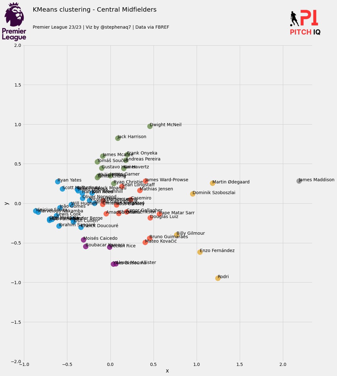
K-Means Clustering for Player Similarity
We perform PCA on the normalized data to reduce its dimensionality while retaining most of the variance. This step helps in simplifying the dataset and identifying the main components that contribute to player performance.
Using the principal components obtained from PCA, we apply K-Means clustering to group players into different clusters based on their performance metrics. This clustering helps in identifying patterns and similarities among players.
def create_kmeans_df(df):
    KMeans_cols = ['Player','Total - Cmp%','KP', 'TB','Sw','PPA', 'PrgP','Tkl%','Blocks', 'Tkl+Int','Clr', 'Carries - PrgDist','SCA90','GCA90','CrsPA','xA', 'Rec','PrgR','xG', 'Sh','SoT']
    df = df[KMeans_cols]
    player_names = df['Player'].tolist()
    df = df.drop(['Player'], axis = 1)
    x = df.values
    scaler = preprocessing.MinMaxScaler()
    x_scaled = scaler.fit_transform(x)
    X_norm = pd.DataFrame(x_scaled)

    pca = PCA(n_components = 2)
    reduced = pd.DataFrame(pca.fit_transform(X_norm))

    wcss = []
    for i in range(1, 11):
        kmeans = KMeans(n_clusters = i, init = 'k-means++', random_state = 42)
        kmeans.fit(reduced)
        wcss.append(kmeans.inertia_)

    kmeans = KMeans(n_clusters=8)
    kmeans = kmeans.fit(reduced)

    labels = kmeans.predict(reduced)
    clusters = kmeans.labels_.tolist()

    reduced['cluster'] = clusters
    reduced['name'] = player_names
    reduced.columns = ['x', 'y', 'cluster', 'name']
    reduced.head()

    return reduced

kmeans_df = create_kmeans_df(key_stats_df)
Explanation:
- Filters the DataFrame for the required columns.
- Extracts player names and normalizes the feature values.
- Reduces the dimensionality of the data using PCA to 2 components.
- Computes Within-Cluster Sum of Squares (WCSS) for 1 to 10 clusters.
- Applies K-Means clustering with 8 clusters.
- Assigns clusters to players and returns a DataFrame with PCA coordinates and cluster assignments.
Finding Similar Players
Certainly! Let’s break down the code find_similar_players and explain the importance of each step:
Function: find_similar_players
def find_similar_players(player_name, df, top_n=15):
    player = df[df['name'] == player_name].iloc[0]
    df['distance'] = np.sqrt((df['x'] - player['x'])**2 + (df['y'] - player['y'])**2)

    max_distance = df['distance'].max()

    df['perc_similarity'] = ((max_distance - df['distance']) / max_distance) * 100

    similar_players = df.sort_values('distance').head(top_n + 1)
    similar_players = similar_players[1:]

    return similar_players
Step-by-Step Explanation
Finding the Player of Interest
player = df[df['name'] == player_name].iloc[0]
Identifying the player of interest from the dataframe (df) based on their name (player_name) is crucial. This step ensures that subsequent calculations and comparisons are focused on the correct player, allowing for accurate similarity analysis.
Calculating Euclidean Distance
df['distance'] = np.sqrt((df['x'] - player['x'])**2 + (df['y'] - player['y'])**2)
Computing the Euclidean distance between the player of interest and all other players in the dataset (df) helps quantify their similarity based on spatial coordinates (x and y). This distance metric is fundamental in determining how close or far players are from each other in a multi-dimensional space.
Normalization of Distance
max_distance = df['distance'].max()
df['perc_similarity'] = ((max_distance - df['distance']) / max_distance) * 100
Normalizing the distance to a percentage scale (perc_similarity) standardizes the comparison of similarity across different players. By normalizing, the function ensures that the most similar players have higher percentage scores, making it easier to interpret and compare their similarity based on distance.
- Selecting Top Similar Players
similar_players = df.sort_values('distance').head(top_n + 1)
similar_players = similar_players[1:]
Importance:
Selecting the top top_n players who are most similar to the player of interest completes the similarity analysis. Sorting the dataframe by distance and excluding the player of interest (who would naturally have a distance of zero) ensures that only truly similar players are included in the final list.
- Returning the Result
return similar_players[['name', 'perc_similarity']]
Returning a dataframe containing the names of similar players along with their percentage similarity scores allows for easy interpretation and further analysis. This output can be directly used for recommendations, clustering analysis, or any other application that requires identifying similar entities based on spatial distance.
The find_similar_players function is important because it enables the identification of players who are spatially closest to a given player in terms of their coordinates (x and y). This functionality is crucial in various applications such as player scouting, team formation, or personalized recommendations in sports analytics. It provides a structured approach to understanding player similarity based on spatial data, which can inform strategic decisions in sports management and analysis.
def find_similar_players(player_name, df, top_n=15):
    player = df[df['name'] == player_name].iloc[0]
    df['distance'] = np.sqrt((df['x'] - player['x'])**2 + (df['y'] - player['y'])**2)

    max_distance = df['distance'].max()

    df['perc_similarity'] = ((max_distance - df['distance']) / max_distance) * 100

    similar_players = df.sort_values('distance').head(top_n + 1)
    similar_players = similar_players[1:]

    return similar_players

similairty_table = find_similar_players(player_name, kmeans_df)[['name','perc_similarity']]
Explanation:
- Finds the player specified by
player_nameand calculates the Euclidean distance to all other players based on PCA coordinates. - Converts distances to a percentage similarity score.
- Sorts players by distance and returns the top N most similar players.
Extracting Key Parameters
params = ['Total - Cmp%','KP', 'PPA', 'PrgP', 'Tkl%', 'Blocks', 'Tkl+Int', 'Clr', 'Carries - PrgDist', 'SCA90', 'xA', 'xG']
Explanation:
- Defines a list of key parameters for player comparison.
Preparing Player Data for Comparison
main_player = pitch_iq_scores[pitch_iq_scores['Player'] == player_name][params].values.tolist()
comp_player_1 = mertrics_similarity

[mertrics_similarity['name'] == similar_player_1][params].values.tolist()
comp_player_2 = mertrics_similarity[mertrics_similarity['name'] == similar_player_2][params].values.tolist()
Explanation:
- Extracts the key parameter values for the main player and two similar players for comparison.
This code is a comprehensive approach to analyzing player performance by preprocessing data, creating scores, normalizing, clustering, and finding similar players. It uses techniques such as Min-Max scaling, PCA, and K-Means clustering.
Normalizing Parameters for Radar Chart
def normalize_list(values_list):
    normalized = []
    for values in values_list:
        min_val = min(values)
        max_val = max(values)
        normalized_values = [(value - min_val) / (max_val - min_val) for value in values]
        normalized.append(normalized_values)
    return normalized

main_player_norm, comp_player_1_norm, comp_player_2_norm = normalize_list([main_player, comp_player_1, comp_player_2])
Explanation:
- Defines a function to normalize each list of parameter values to a 0-1 range.
- Normalizes the parameter values for the main player and the two comparison players.
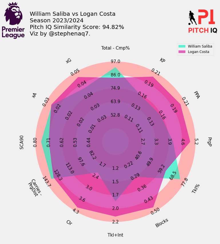
Setting Up for Radar Chart Visualization
import matplotlib.pyplot as plt
import numpy as np

params = ['Total - Cmp%', 'KP', 'PPA', 'PrgP', 'Tkl%', 'Blocks', 'Tkl+Int', 'Clr', 'Carries - PrgDist', 'SCA90', 'xA', 'xG']
num_vars = len(params)

angles = np.linspace(0, 2 * np.pi, num_vars, endpoint=False).tolist()
angles += angles[:1]

def plot_radar_chart(names, values, title):
    fig, ax = plt.subplots(figsize=(8, 8), subplot_kw=dict(polar=True))
    ax.set_theta_offset(np.pi / 2)
    ax.set_theta_direction(-1)
    plt.xticks(angles[:-1], params, color='grey', size=8)
    ax.set_rscale('log')

    for name, value in zip(names, values):
        values = value + value[:1]
        ax.plot(angles, values, linewidth=2, linestyle='solid', label=name)
        ax.fill(angles, values, alpha=0.25)

    plt.legend(loc='upper right', bbox_to_anchor=(0.1, 0.1))
    plt.title(title, size=20, color='grey', y=1.1)
    plt.show()

names = [player_name, similar_player_1, similar_player_2]
values = [main_player_norm[0], comp_player_1_norm[0], comp_player_2_norm[0]]

plot_radar_chart(names, values, 'Player Comparison')
Complete Code Integration
The code integrates various steps to preprocess data, create metric scores, normalize values, cluster players, find similar players, normalize key parameters, and visualize the results in a radar chart. Here is how the complete code looks when put together:
-
Imports: Imports necessary libraries such as
pandas,numpy,matplotlib, andsklearnfor data processing, visualization, and machine learning. - Key Statistics Preprocessing:
- Filters and preprocesses the key statistics for players based on position and removes rows with any
NaNvalues. - Converts the statistics to per 90-minute values.
- Filters and preprocesses the key statistics for players based on position and removes rows with any
- Metrics Scores Creation:
- Normalizes the core statistics and computes scores for passing, defending, creation, and shooting metrics.
- Adjust Player Rating Range:
- Adjusts the rating range for player scores to a specified range.
- K-Means Clustering:
- Normalizes data, reduces dimensionality using PCA, and applies K-Means clustering to group similar players.
- Assigns cluster labels to players.
- Finding Similar Players:
- Computes the distance of each player from the target player in the reduced feature space.
- Determines the similarity percentage and identifies the top similar players.
- Normalizing Parameters:
- Normalizes the parameter values for the radar chart.
- Radar Chart Visualization:
- Sets up the parameters and angles for the radar chart.
- Defines a function to plot the radar chart, comparing the main player with the two most similar players.
This comprehensive approach enables detailed player performance analysis, similarity comparison, and effective visualization using a radar chart.
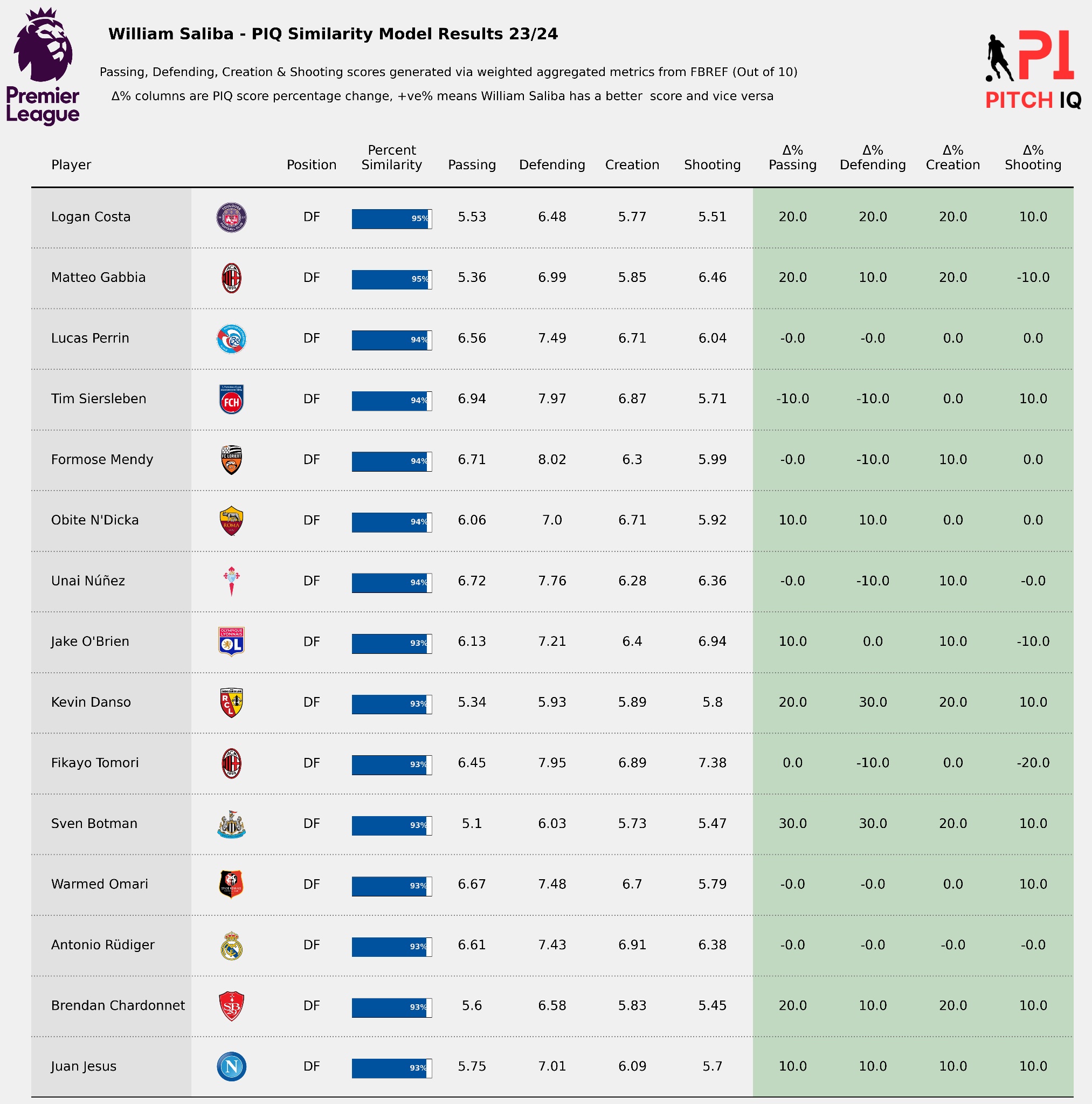
Here are the top 5 players that profile most closely to William Saliba:
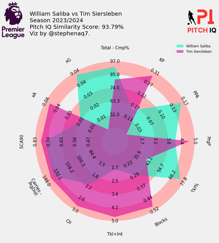
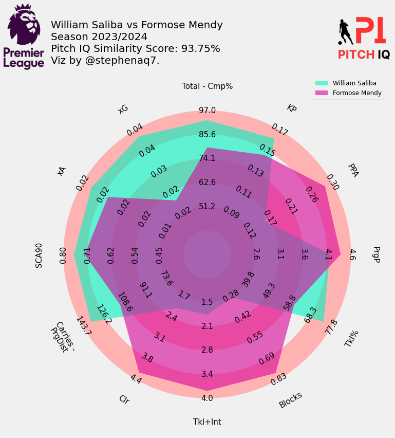
When Putting it all together, I have created a final visual, showing the top 15 most similar players to Saliba in a handy table.
Conclusion
In conclusion, this post serves as a valuable addition to a series of tutorials aimed at empowering users to utitlizie data science techniques to better understand manipulate data available from FBREF as well as generating insightful data visualizations,and brief introduction into using python libraries such as sk.learn.
Thanks for reading
Steve

Comments