53 min to read
K-Means Player Cluster Analysis
Analyzing and categorizing football player roles through clustering
Introduction
In this post, we undertake an exploration into the application of the K-means clustering algorithm, a fundamental unsupervised machine learning approach.
K-means clustering serves as a pivotal method in vector quantization, striving to segregate a given dataset into distinct clusters, where each datum is assigned to the cluster with the nearest centroid.
In other words, K-means is able to find relationships in data and create groups of similar characteristics.
This technique facilitates the extraction of latent patterns within the data, thus facilitating the categorization of analogous attributes.
Background on K-Means
K-Means aims to group similar data points together while keeping dissimilar points apart. The algorithm works by iteratively assigning each data point to the nearest cluster centroid and then recalculating the centroids based on the mean of the data points in each cluster. This process continues until the centroids stabilize or a predefined number of iterations is reached. K-means is widely used in various fields such as data mining, image segmentation, and customer segmentation for its simplicity and effectiveness in identifying patterns within data.
The key steps in K means can be broken down into the following:
1) Partitioning: K-means clustering partitions a dataset into a predetermined number of clusters (k) based on the similarity of data points.
2) Centroid Initialization: Initially, k centroids are randomly placed in the feature space, representing the center of each cluster.
3) Assignment: Each data point is assigned to the cluster whose centroid is closest in terms of Euclidean distance.
4) Centroid Update: After all data points are assigned, the centroids are recalculated as the mean of all points within each cluster.
5) Convergence: The assignment and centroid update steps are iteratively performed until convergence, i.e., until the centroids no longer change significantly or a maximum number of iterations is reached.
K-means clustering is used for various reasons:
1) Data Exploration: It helps to understand the structure of the data by grouping similar data points together, which can reveal underlying patterns and relationships.
2) Pattern Recognition: K-means can identify clusters within data that may not be immediately apparent, making it useful for pattern recognition tasks.
3) Data Compression: By reducing the dimensionality of the data through clustering, K-means can help in data compression, making it easier to visualize and analyze large datasets.
4) Segmentation: It is widely used for customer segmentation in marketing, where it helps to divide customers into distinct groups based on their characteristics or behaviors.
5) Preprocessing: K-means clustering can be used as a preprocessing step for other machine learning algorithms, such as classification or regression, by reducing the complexity of the data and improving the performance of these models.
In this post we’re going to tain the K Means algorithm on a dataset that I scraped from FBREF. A detailed tutorial of how to do so can be found here.
Setup
Here are some of the key modules that are required in order to run this script. This Python script imports libraries for web scraping, data analysis, visualization, and machine learning. It configures the visualization environment, sets display options, and imports image processing modules.
The KMeans module is utilized for performing K-means clustering. The preprocessing module provides functionality for preparing data by scaling, centering, or transforming it before applying machine learning algorithms. PCA, accessible through the decomposition submodule, is a technique for dimensionality reduction, often employed to visualize high-dimensional data or reduce computational complexity. Lastly, the MinMaxScaler module scales features to a given range, typically between 0 and 1, a preprocessing step often employed to improve algorithm performance. These modules collectively facilitate data preprocessing, clustering, and dimensionality reduction, which are fundamental steps in many machine learning workflows.
import os
import requests
import pandas as pd
from bs4 import BeautifulSoup
import seaborn as sb
import matplotlib.pyplot as plt
import matplotlib as mpl
import warnings
import numpy as np
from math import pi
from urllib.request import urlopen
import matplotlib.patheffects as pe
from highlight_text import fig_text
from adjustText import adjust_text
from tabulate import tabulate
import matplotlib.style as style
import unicodedata
from fuzzywuzzy import fuzz
from fuzzywuzzy import process
import matplotlib.ticker as ticker
import matplotlib.patheffects as path_effects
import matplotlib.font_manager as fm
import matplotlib.colors as mcolors
from matplotlib import cm
from highlight_text import fig_text

import matplotlib.pyplot as plt
import seaborn as sns
%matplotlib inline

from sklearn.cluster import KMeans
from sklearn import preprocessing
from sklearn.decomposition import PCA
from sklearn.preprocessing import MinMaxScaler

style.use('fivethirtyeight')

from PIL import Image
import urllib
import os
import math
from PIL import Image
import matplotlib.image as image
pd.options.display.max_columns = None
Data Preparation & Constructing Functions
This section can also be found in my other tutorial here - FBREF Data Scraping Pt.4:
The code below defines a function called position_grouping that takes a player’s position (x) as input. It categorizes players into different position groups based on their positions, such as goalkeepers (GK), defenders, wing-backs, defensive midfielders, central midfielders, attacking midfielders, and forwards.
The function uses conditional statements (if-elif-else) to determine the appropriate position group for a given input position. If the input matches any predefined positions for a group, it returns the corresponding group name. If the position doesn’t match any predefined groups, it returns “unidentified position.” The purpose is to classify football players into broader position categories for easier analysis or grouping.
keepers = ['GK']
defenders = ["DF",'DF,MF']
wing_backs = ['FW,DF','DF,FW']
defensive_mids = ['MF,DF']
midfielders = ['MF']
attacking_mids = ['MF,FW',"FW,MF"]
forwards = ['FW']

def position_grouping(x):
    if x in keepers:
        return "GK"
    elif x in defenders:
        return "Defender"
    elif x in wing_backs:
        return "Wing-Back"
    elif x in defensive_mids:
        return "Defensive-Midfielders"
    elif x in midfielders:
        return "Central Midfielders"
    elif x in attacking_mids:
        return "Attacking Midfielders"
    elif x in forwards:
        return "Forwards"
    else:
        return "unidentified position"
The next code block is basis upon which we will use to build our database creator function. I will use the pass metrics pages as the example -
This code starts by scraping passing statistics from a specified URL using the requests library and parsing the HTML content with BeautifulSoup.
The HTML content is then cleaned to remove comments and stored as a string.
The cleaned HTML content is read into a pandas DataFrame using pd.read_html().
The script modifies the DataFrame to handle multi-level column headers and assigns appropriate prefixes to distinguish passing metrics (Total, Short, Medium, Long).
Finally, it filters out rows where the ‘Player’ column is not populated, likely removing headers and irrelevant information, to prepare the DataFrame for further analysis.
    # Passing columns
pass_ = 'https://fbref.com/en/comps/9/passing/Premier-League-Stats'
page =requests.get(pass_)
soup = BeautifulSoup(page.content, 'html.parser')
html_content = requests.get(pass_).text.replace('<!--', '').replace('-->', '')
pass_df = pd.read_html(html_content)
pass_df[-1].columns = pass_df[-1].columns.droplevel(0)
pass_stats = pass_df[-1]
pass_prefixes = {1: 'Total - ', 2: 'Short - ', 3: 'Medium - ', 4: 'Long - '}
pass_column_occurrences = {'Cmp': 0, 'Att': 0, 'Cmp%': 0}
pass_new_column_names = []
for col_name in pass_stats.columns:
    if col_name in pass_column_occurrences:
        pass_column_occurrences[col_name] += 1
        prefix = pass_prefixes[pass_column_occurrences[col_name]]
        pass_new_column_names.append(prefix + col_name)
    else:
        pass_new_column_names.append(col_name)
pass_stats.columns = pass_new_column_names
pass_stats = pass_stats[pass_stats['Player'] != 'Player']
This Python function create_full_stats_db() retrieves various football statistics from different URLs, cleans and processes the data, and merges them into a single DataFrame for comprehensive analysis:
1: Passing Statistics: Retrieves passing data from a URL, processes it to handle multi-level column headers, and renames columns with appropriate prefixes.
2: Shooting Statistics: Fetches shooting data, cleans it by dropping irrelevant rows, and stores it.
3: Passing Type Statistics: Gathers passing type data, cleans column headers, and stores it.
4: Goal Creation & Assists Statistics (GCA): Fetches GCA data, processes column headers, and stores it.
4: Defensive Statistics: Retrieves defensive data, renames columns, and stores it.
5: Possession Statistics: Gathers possession-related data, renames columns, and stores it.
6: Miscellaneous Statistics: Retrieves miscellaneous data, cleans it, and stores it.
7: Merging DataFrames: Merges all the data frames on common player attributes, such as name, nationality, position, squad, age, and playing time.
8: Data Cleaning: Handles missing values, converts non-numeric columns to numeric where possible, and adds a column for position grouping using the previously defined position_grouping function.
9: Returns: Returns the merged and cleaned DataFrame containing all the football statistics for further analysis.
Here is the full function below:
def create_full_stats_db():
    # Passing columns
    pass_ = 'https://fbref.com/en/comps/9/passing/Premier-League-Stats'
    page =requests.get(pass_)
    soup = BeautifulSoup(page.content, 'html.parser')
    html_content = requests.get(pass_).text.replace('<!--', '').replace('-->', '')
    pass_df = pd.read_html(html_content)
    pass_df[-1].columns = pass_df[-1].columns.droplevel(0)
    pass_stats = pass_df[-1]
    pass_prefixes = {1: 'Total - ', 2: 'Short - ', 3: 'Medium - ', 4: 'Long - '}
    pass_column_occurrences = {'Cmp': 0, 'Att': 0, 'Cmp%': 0}
    pass_new_column_names = []
    for col_name in pass_stats.columns:
        if col_name in pass_column_occurrences:
            pass_column_occurrences[col_name] += 1
            prefix = pass_prefixes[pass_column_occurrences[col_name]]
            pass_new_column_names.append(prefix + col_name)
        else:
            pass_new_column_names.append(col_name)
    pass_stats.columns = pass_new_column_names
    pass_stats = pass_stats[pass_stats['Player'] != 'Player']

    # Shooting columns
    shot_ = 'https://fbref.com/en/comps/9/shooting/Premier-League-Stats'
    page =requests.get(shot_)
    soup = BeautifulSoup(page.content, 'html.parser')
    html_content = requests.get(shot_).text.replace('<!--', '').replace('-->', '')
    shot_df = pd.read_html(html_content)
    shot_df[-1].columns = shot_df[-1].columns.droplevel(0) # drop top header row
    shot_stats = shot_df[-1]
    shot_stats = shot_stats[shot_stats['Player'] != 'Player']


    # Pass Type columns
    pass_type = 'https://fbref.com/en/comps/9/passing_types/Premier-League-Stats'
    page =requests.get(pass_type)
    soup = BeautifulSoup(page.content, 'html.parser')
    html_content = requests.get(pass_type).text.replace('<!--', '').replace('-->', '')
    pass_type_df = pd.read_html(html_content)
    pass_type_df[-1].columns = pass_type_df[-1].columns.droplevel(0) # drop top header row
    pass_type_stats = pass_type_df[-1]
    pass_type_stats = pass_type_stats[pass_type_stats['Player'] != 'Player']


    # GCA columns
    gca_ = 'https://fbref.com/en/comps/9/gca/Premier-League-Stats'
    page =requests.get(gca_)
    soup = BeautifulSoup(page.content, 'html.parser')
    html_content = requests.get(gca_).text.replace('<!--', '').replace('-->', '')
    gca_df = pd.read_html(html_content)
    gca_df[-1].columns = gca_df[-1].columns.droplevel(0)
    gca_stats = gca_df[-1]
    gca_prefixes = {1: 'SCA - ', 2: 'GCA - '}
    gca_column_occurrences = {'PassLive': 0, 'PassDead': 0, 'TO%': 0, 'Sh': 0, 'Fld': 0, 'Def': 0}
    gca_new_column_names = []
    for col_name in gca_stats.columns:
        if col_name in gca_column_occurrences:
            gca_column_occurrences[col_name] += 1
            prefix = gca_prefixes[gca_column_occurrences[col_name]]
            gca_new_column_names.append(prefix + col_name)
        else:
            gca_new_column_names.append(col_name)
    gca_stats.columns = gca_new_column_names
    gca_stats = gca_stats[gca_stats['Player'] != 'Player']


    # Defense columns
    defence_ = 'https://fbref.com/en/comps/9/defense/Premier-League-Stats'
    page =requests.get(defence_)
    soup = BeautifulSoup(page.content, 'html.parser')
    html_content = requests.get(defence_).text.replace('<!--', '').replace('-->', '')
    defence_df = pd.read_html(html_content)
    defence_df[-1].columns = defence_df[-1].columns.droplevel(0) # drop top header row
    defence_stats = defence_df[-1]
    rename_columns = {
    'Def 3rd': 'Tackles - Def 3rd',
    'Mid 3rd': 'Tackles - Mid 3rd',
    'Att 3rd': 'Tackles - Att 3rd',
    'Blocks': 'Total Blocks',
    'Sh': 'Shots Blocked',
    'Pass': 'Passes Blocked'}
    defence_stats.rename(columns = rename_columns, inplace=True)
    defence_prefixes = {1: 'Total - ', 2: 'Dribblers- '}
    defence_column_occurrences = {'Tkl': 0}
    new_column_names = []
    for col_name in defence_stats.columns:
        if col_name in defence_column_occurrences:
            defence_column_occurrences[col_name] += 1
            prefix = defence_prefixes[defence_column_occurrences[col_name]]
            new_column_names.append(prefix + col_name)
        else:
            new_column_names.append(col_name)
    defence_stats.columns = new_column_names
    defence_stats = defence_stats[defence_stats['Player'] != 'Player']


    # possession columns
    poss_ = 'https://fbref.com/en/comps/9/possession/Premier-League-Stats'
    page =requests.get(poss_)
    soup = BeautifulSoup(page.content, 'html.parser')
    html_content = requests.get(poss_).text.replace('<!--', '').replace('-->', '')
    poss_df = pd.read_html(html_content)
    poss_df[-1].columns = poss_df[-1].columns.droplevel(0) # drop top header row
    poss_stats = poss_df[-1]
    rename_columns = {
    'TotDist': 'Carries - TotDist',
    'PrgDist': 'Carries - PrgDist',
    'PrgC': 'Carries - PrgC',
    '1/3': 'Carries - 1/3',
    'CPA': 'Carries - CPA',
    'Mis': 'Carries - Mis',
    'Dis': 'Carries - Dis',
    'Att': 'Take Ons - Attempted'  }
    poss_stats.rename(columns=rename_columns, inplace=True)
    poss_stats = poss_stats[poss_stats['Player'] != 'Player']


    # misc columns
    misc_ = 'https://fbref.com/en/comps/9/misc/Premier-League-Stats'
    page =requests.get(misc_)
    soup = BeautifulSoup(page.content, 'html.parser')
    html_content = requests.get(misc_).text.replace('<!--', '').replace('-->', '')
    misc_df = pd.read_html(html_content)
    misc_df[-1].columns = misc_df[-1].columns.droplevel(0) # drop top header row
    misc_stats = misc_df[-1]
    misc_stats = misc_stats[misc_stats['Player'] != 'Player']

    index_df = misc_stats[['Player', 'Nation', 'Pos', 'Squad', 'Age', 'Born', '90s']]

    data_frames = [poss_stats, misc_stats, pass_stats ,defence_stats, shot_stats, gca_stats, pass_type_stats]
    for df in data_frames:
        if df is not None:  # Checking if the DataFrame exists
            df.drop(columns=['Matches', 'Rk'], inplace=True, errors='ignore')
            df.dropna(axis=0, how='any', inplace=True)

            index_df = pd.merge(index_df, df, on=['Player', 'Nation', 'Pos', 'Squad', 'Age', 'Born', '90s'], how='left')
    index_df["position_group"] = index_df.Pos.apply(lambda x: position_grouping(x))

    index_df.fillna(0, inplace=True)

    non_numeric_cols = ['Player', 'Nation', 'Pos', 'Squad', 'Age', 'position_group']

    def clean_non_convertible_values(value):
        try:
            return pd.to_numeric(value)
        except (ValueError, TypeError):
            return np.nan

    # Iterate through each column, converting non-numeric columns to numeric
    for col in index_df.columns:
        if col not in non_numeric_cols:
            index_df[col] = index_df[col].apply(clean_non_convertible_values)


    return index_df
Now that we have our function, we can now store all of the relevant pages as variables and pass them into out function arguments of the function. The variables can be stored as follows:
fbref_passing = 'https://fbref.com/en/comps/Big5/passing/players/Big-5-European-Leagues-Stats'
fbref_shooting = 'https://fbref.com/en/comps/Big5/shooting/players/Big-5-European-Leagues-Stats'
fbref_pass_type = 'https://fbref.com/en/comps/Big5/passing_types/players/Big-5-European-Leagues-Stats'
fbref_defence = 'https://fbref.com/en/comps/Big5/defense/players/Big-5-European-Leagues-Stats'
fbref_gca = 'https://fbref.com/en/comps/Big5/gca/players/Big-5-European-Leagues-Stats'
fbref_poss = 'https://fbref.com/en/comps/Big5/possession/players/Big-5-European-Leagues-Stats'
fbref_misc = 'https://fbref.com/en/comps/Big5/misc/players/Big-5-European-Leagues-Stats'
stats = create_full_stats_db(fbref_passing,fbref_shooting,fbref_pass_type,fbref_defence,fbref_gca,fbref_poss,fbref_misc)
We have now created a relatively simple function that is able to retrieve all key player data from FBREF in under 11 seconds, meaning that this data can easily be refreshed with minimal effort.
This next code block comprises of a function that essentially performs a per-90-minute normalization for numeric columns in the DataFrame, excluding certain columns and handling division by zero cases.
Here’s a breakdown of the code per_90fi:
1: Fill NaN Values:
- Replaces all NaN values in the DataFrame with 0.
dataframe = dataframe.fillna(0)
2: Identify Numeric Columns:
- Finds all columns in the DataFrame that contain numeric data.
numeric_columns = [col for col in dataframe.columns if np.issubdtype(dataframe[col].dtype, np.number)]
3: Exclude Columns:
- Specifies columns to exclude from normalization, such as player names, nationality, position, squad, age, birth year, position group, and the column ’90s’ (presumably representing minutes played).
exclude_columns = ['Player', 'Nation', 'Pos', 'Squad', 'Age', 'Born', 'position_group','90s']
4: Identify Columns to Divide:
- Identifies numeric columns to divide by the ’90s’ column.
- Excludes columns containing ‘90’ or ‘%’ in their names.
   columns_to_divide = [col for col in numeric_columns if col not in exclude_columns
                         and '90' not in col and '%' not in col and '90s' not in col]
5: Create a Mask:
- Creates a boolean mask to avoid division by zero or blank values for the ’90s’ column.
mask = (dataframe['90s'] != 0)
6: Normalize Data:
- Divides each identified column by the ’90s’ column, handling division by zero or blank values.
   for col in columns_to_divide:
       dataframe.loc[mask, col] /= dataframe.loc[mask, '90s']
7: Return DataFrame:
- Returns the modified DataFrame after normalization.
Here is the full code below:
def per_90fi(dataframe):
    # Replace empty strings ('') with NaN
    dataframe = dataframe.replace('', np.nan)

    # Fill NaN values with 0
    dataframe = dataframe.fillna(0)

    # Identify numeric columns excluding '90s' and columns with '90' or '%' in their names
    exclude_columns = ['Player', 'Nation', 'Pos', 'Squad', 'Age', 'Born', 'position_group']
    numeric_columns = [col for col in dataframe.columns if np.issubdtype(dataframe[col].dtype, np.number)
                       and col != '90s' and not any(exc_col in col for exc_col in exclude_columns)
                       and ('90' not in col) and ('%' not in col)]

    # Create a mask to avoid division by zero
    mask = (dataframe['90s'] != 0)

    # Divide each numeric column by the '90s' column row-wise
    dataframe.loc[mask, numeric_columns] = dataframe.loc[mask, numeric_columns].div(dataframe.loc[mask, '90s'], axis=0)

    return dataframe
position = "Defender"
stats = create_full_stats_db(fbref_passing,fbref_shooting,fbref_pass_type,fbref_defence,fbref_gca,fbref_poss,fbref_misc)

def key_stats_db(df,position):
    non_numeric_cols = ['Player', 'Nation', 'Pos', 'Squad', 'Age', 'position_group']
    core_stats = ['90s','Total - Cmp%','KP', 'TB','Sw','PPA', 'PrgP','Tkl%','Blocks_x', 'Tkl+Int','Clr', 'Carries - PrgDist','SCA90','GCA90','CrsPA','xA', 'Rec','PrgR','xG', 'Sh','SoT']
    df.dropna(axis=0, how='any', inplace=True)
    key_stats_df = df[df['position_group'] == position]
    key_stats_df = key_stats_df[non_numeric_cols + core_stats]
    key_stats_df = key_stats_df[key_stats_df['90s'] > 5]
    key_stats_df = per_90fi(key_stats_df)
    return key_stats_df


key_stats_df = key_stats_db(stats,position)
The provided code below is designed to create and adjust performance scores for football players based on various key statistics. Initially, the code defines groups of metrics related to different aspects of player performance such as passing, defending, creation, and shooting.
It then proceeds to normalize these metrics using a Min-Max scaling technique, ensuring that they fall within a common range for comparison purposes.
Subsequently, the code calculates performance scores for each player based on their normalized metrics, assigning scores for passing, defending, creation, and shooting abilities.
To ensure uniqueness, a small offset is added to each score. Finally, the code adjusts the player ratings to fit within a desired range and merges the newly computed scores with the original dataset containing the player statistics.
Here are the steps with the corresponding code blocks:
1) Define Metric Groups:
Define separate lists for core statistics, passing metrics, defending metrics, creation metrics, and shooting metrics based on their relevance in the analysis.
   core_stats = ['90s','Total - Cmp%','KP', 'TB','Sw','PPA', 'PrgP','Tkl%','Blocks_x', 'Tkl+Int','Clr', 'Carries - PrgDist','SCA90','GCA90','CrsPA','xA', 'Rec','PrgR','xG', 'Sh','SoT']
   passing_metrics = ['Total - Cmp%', 'KP', 'TB', 'Sw', 'PPA', 'PrgP']
   defending_metrics = ['Tkl%', 'Blocks_x', 'Tkl+Int', 'Clr']
   creation_metrics = ['Carries - PrgDist', 'SCA90', 'GCA90', 'CrsPA', 'xA', 'Rec', 'PrgR']
   shooting_metrics = ['xG', 'Sh', 'SoT']
2) Normalize Data:
Instantiate a MinMaxScaler to normalize the core statistics in the provided DataFrame key_stats_df. This ensures that each metric is on the same scale for fair comparison.
   scaler = MinMaxScaler()
   stats_normalized = key_stats_df.copy()
   stats_normalized[core_stats] = scaler.fit_transform(stats_normalized[core_stats])
3) Calculate Scores:
Calculate average scores for passing, defending, creation, and shooting metrics for each player in the DataFrame. These scores represent the performance of players in different aspects of the game, scaled to a range of 0 to 10 for easy interpretation and comparison.
   stats_normalized['Passing_Score'] = stats_normalized[passing_metrics].mean(axis=1) * 10
   stats_normalized['Defending_Score'] = stats_normalized[defending_metrics].mean(axis=1) * 10
   stats_normalized['Creation_Score'] = stats_normalized[creation_metrics].mean(axis=1) * 10
   stats_normalized['Shooting_Score'] = stats_normalized[shooting_metrics].mean(axis=1) * 10
4) Add Offset:
Add a small offset to each score to ensure uniqueness among players with identical metric averages. This helps avoid conflicts when merging or processing the data further.
   stats_normalized['Passing_Score'] += stats_normalized.index * 0.001
   stats_normalized['Defending_Score'] += stats_normalized.index * 0.001
   stats_normalized['Creation_Score'] += stats_normalized.index * 0.001
   stats_normalized['Shooting_Score'] += stats_normalized.index * 0.001
5) Clip Scores:
Ensure that all scores fall within the range of 0 to 10 by clipping any values outside this range. This step guarantees consistency and meaningfulness of the scores.
stats_normalized[['Passing_Score', 'Defending_Score', 'Creation_Score', 'Shooting_Score']] = stats_normalized[['Passing_Score', 'Defending_Score', 'Creation_Score', 'Shooting_Score']].clip(lower=0, upper=10)
6) Adjust Player Ratings:
Define a function adjust_player_rating_range to normalize player ratings to a desired range (in this case, 4.5 to 9.5). This step ensures that player ratings are within a specific range for consistency and ease of interpretation.
   player_ratings = dataframe[['Passing_Score', 'Defending_Score', 'Creation_Score', 'Shooting_Score']]
   min_rating = 4.5
   max_rating = 9.5
   for col in player_ratings.columns:
       normalized_ratings = min_rating + (max_rating - min_rating) * ((player_ratings[col] - player_ratings[col].min()) / (player_ratings[col].max() - player_ratings[col].min()))
       dataframe[col] = normalized_ratings
7) Apply Functions:
Apply the defined functions create_metrics_scores and adjust_player_rating_range to the DataFrame key_stats_df to compute the pitch IQ scores for each player and adjust their ratings accordingly.
   pitch_iq_scoring = create_metrics_scores(key_stats_df)
   pitch_iq_scoring = adjust_player_rating_range(pitch_iq_scoring)
8) Merge DataFrames:
Merge the resulting DataFrame containing pitch IQ scores with the original key_stats_df DataFrame based on the ‘Player’ column to incorporate the computed scores into the dataset for further analysis.
pitch_iq_scores = pd.merge(key_stats_df, pitch_iq_scoring, on='Player', how='left')
This is how the full code is constructed:
def create_metrics_scores(key_stats_df):
    # Define the key_stats grouped by the metrics
    core_stats = ['90s','Total - Cmp%','KP', 'TB','Sw','PPA', 'PrgP','Tkl%','Blocks_x', 'Tkl+Int','Clr', 'Carries - PrgDist','SCA90','GCA90','CrsPA','xA', 'Rec','PrgR','xG', 'Sh','SoT']
    passing_metrics = ['Total - Cmp%', 'KP', 'TB', 'Sw', 'PPA', 'PrgP']
    defending_metrics = ['Tkl%', 'Blocks_x', 'Tkl+Int', 'Clr']
    creation_metrics = ['Carries - PrgDist', 'SCA90', 'GCA90', 'CrsPA', 'xA', 'Rec', 'PrgR']
    shooting_metrics = ['xG', 'Sh', 'SoT']

    # Create a MinMaxScaler instance
    scaler = MinMaxScaler()

    # Normalize the metrics
    stats_normalized = key_stats_df.copy()  # Create a copy of the DataFrame
    stats_normalized[core_stats] = scaler.fit_transform(stats_normalized[core_stats])

    # Calculate scores for each metric grouping and scale to 0-10
    stats_normalized['Passing_Score'] = stats_normalized[passing_metrics].mean(axis=1) * 10
    stats_normalized['Defending_Score'] = stats_normalized[defending_metrics].mean(axis=1) * 10
    stats_normalized['Creation_Score'] = stats_normalized[creation_metrics].mean(axis=1) * 10
    stats_normalized['Shooting_Score'] = stats_normalized[shooting_metrics].mean(axis=1) * 10

    # Add a small offset to ensure unique scores
    stats_normalized['Passing_Score'] += stats_normalized.index * 0.001
    stats_normalized['Defending_Score'] += stats_normalized.index * 0.001
    stats_normalized['Creation_Score'] += stats_normalized.index * 0.001
    stats_normalized['Shooting_Score'] += stats_normalized.index * 0.001

    # Clip scores to ensure they are within the 0-10 range
    stats_normalized[['Passing_Score', 'Defending_Score', 'Creation_Score', 'Shooting_Score']] = stats_normalized[['Passing_Score', 'Defending_Score', 'Creation_Score', 'Shooting_Score']].clip(lower=0, upper=10)
    return stats_normalized

def adjust_player_rating_range(dataframe):
    # Get the 'total player rating' column
    player_ratings = dataframe[['Passing_Score', 'Defending_Score', 'Creation_Score', 'Shooting_Score']]

    # Define the desired range for the ratings
    min_rating = 4.5
    max_rating = 9.5

    # Normalize the ratings to be within the desired range (5 to 9.5) for each column
    for col in player_ratings.columns:
        normalized_ratings = min_rating + (max_rating - min_rating) * ((player_ratings[col] - player_ratings[col].min()) / (player_ratings[col].max() - player_ratings[col].min()))
        dataframe[col] = normalized_ratings

    return dataframe


pitch_iq_scoring = create_metrics_scores(key_stats_df)
pitch_iq_scoring = adjust_player_rating_range(pitch_iq_scoring)
pitch_iq_scoring = pitch_iq_scoring[['Player','Passing_Score', 'Defending_Score', 'Creation_Score', 'Shooting_Score']]
pitch_iq_scores = pd.merge(key_stats_df, pitch_iq_scoring, on='Player', how='left')
2-D KMeans Analysis
Here we’ll use PCA as a way to reduce our dimensions. Let’s scale it down to 2 dimensions so we can see the data in a 2D plot with the K-means results.
Principal Component Analysis (PCA) serves as a pivotal preprocessing step for various data analysis tasks, one of which is the K-means clustering algorithm. In the realm of 2D K-means analysis, where the objective is to partition a dataset into distinct clusters in a two-dimensional space, PCA emerges as an indispensable tool for dimensionality reduction and data visualization.
By condensing the information from the original feature space into a lower-dimensional representation while preserving the essential variance, PCA not only facilitates more efficient computation but also enhances the interpretability of clustering results.
This combination of PCA and 2D K-means holds immense value in uncovering underlying structures, patterns, and relationships within datasets, thus aiding in insightful data exploration and decision-making.
The code below performs K-means clustering analysis on a dataset using a subset of columns (‘KMeans_cols’) from ‘key_stats_df’.
Here’s a breakdown of each step:
1: Column Selection: ‘KMeans_cols’ specifies the columns to be used in the analysis. These columns likely represent various statistics or features related to players in a sports context.
2: Data Preparation:
- ‘df’ is created by selecting only the columns specified in ‘KMeans_cols’.
- ‘player_names’ is a list containing the names of the players.
- ‘df’ is then modified to remove the ‘Player’ column, as it’s not used in the subsequent analysis.
3: Normalization:
- The data in ‘df’ is normalized using Min-Max scaling to ensure that all features are on the same scale. This step is crucial for PCA, as it requires standardized data to calculate principal components accurately.
- ‘preprocessing.MinMaxScaler()’ is used for normalization.
- ‘x_scaled’ contains the normalized data.
4: Principal Component Analysis (PCA):
- PCA is applied to reduce the dimensionality of the dataset while preserving the most important information.
- ‘PCA(n_components = 2)’ specifies that the transformed data should be reduced to 2 dimensions.
- ‘pca.fit_transform(X_norm)’ performs PCA on the normalized data and returns the transformed data, which is then stored in ‘reduced’.
- ‘reduced’ is a DataFrame containing the principal components of the original dataset.
After executing this code, ‘reduced’ will contain the transformed data with reduced dimensionality, suitable for further analysis such as clustering using K-means algorithm in 2D space. Each row in ‘reduced’ corresponds to a player, with their statistical features transformed into two principal components. These components represent combinations of the original features that capture the most significant variance in the data.
KMeans_cols = ['Player','Total - Cmp%','KP', 'TB','Sw','PPA', 'PrgP','Tkl%','Blocks_x', 'Tkl+Int','Clr', 'Carries - PrgDist','SCA90','GCA90','CrsPA','xA', 'Rec','PrgR','xG', 'Sh','SoT']
df = key_stats_df[KMeans_cols]
player_names = df['Player'].tolist()
df = df.drop(['Player'], axis = 1)
x = df.values
scaler = preprocessing.MinMaxScaler()
x_scaled = scaler.fit_transform(x)
X_norm = pd.DataFrame(x_scaled)
pca = PCA(n_components = 2)
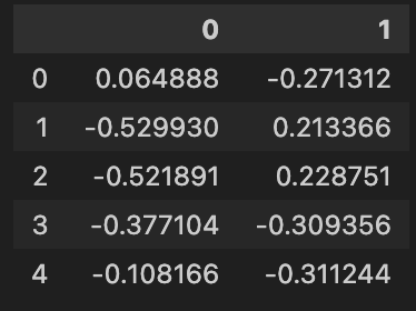
reduced = pd.DataFrame(pca.fit_transform(X_norm))
After executing this code, ‘reduced’ will contain the transformed data with reduced dimensionality, suitable for further analysis such as clustering using K-means algorithm in 2D space. Each row in ‘reduced’ corresponds to a player, with their statistical features transformed into two principal components. These components represent combinations of the original features that capture the most significant variance in the data.
Here’s a constrained view of the output:
Now that we’ve utilized PCA to reduce the dimensions of our dataset, we can generate a 2D plot to visualize the relationships among our players. However, it’s important to note that this plot merely represents similarities between players, as the principal components (PC1 and PC2) derived from PCA aren’t directly interpretable by technical or scouting teams.
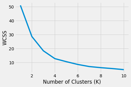
With our 2D similarity metric in hand, we can proceed to apply the K-means algorithm to cluster players based on their similarities. However, before doing so, we need to determine the optimal number of clusters (K) for our analysis. To achieve this, we employ a method called the Elbow method, which is implemented below. This involves training multiple K-means models with varying numbers of clusters (from 1 to 11), and calculating the Within-Cluster Sum of Squares (WCSS) for each model.
WCSS quantifies the sum of squared distances between each data point and its respective cluster centroid. This metric serves as a measure of the compactness of the clusters.
wcss = []
for i in range(1, 11):
    kmeans = KMeans(n_clusters = i, init = 'k-means++', random_state = 42)
    kmeans.fit(reduced)
    wcss.append(kmeans.inertia_)
kmeans = KMeans(n_clusters=6)
kmeans = kmeans.fit(reduced)
labels = kmeans.predict(reduced)
clusters = kmeans.labels_.tolist()
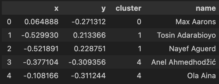
reduced['cluster'] = clusters
reduced['name'] = player_names
reduced.columns = ['x', 'y', 'cluster', 'name']
reduced.head()
According to the elbow method, we determine that K=6, identified as the point where the rate of decrease in WCSS slows down significantly on our graph.
Now, let’s proceed to train a K-means model for K=6 and observe its performance.
After training and using the trained model, each player in the dataset now has a number from 0 to 5 that represents their set. Let’s put this information in our reduced dataset and then plot it with the results of K-means.
In order to quickly reproduce this model against another dataset if need be for later use, I’ve wrapped the code above into an easy to use function.
The code effectively preprocesses the data, performs dimensionality reduction using PCA, determines the optimal number of clusters using the elbow method, and applies K-means clustering to group players into clusters based on their statistics. Finally, it returns a DataFrame containing the reduced data with cluster labels and player names.
Here is brief summary of the steps:
1: Column Selection:
- Define a list of columns called
KMeans_colsthat includes player names and various statistics related to them. - Extract only the specified columns from the input DataFrame
df.
2: Data Preparation:
- Extract player names from the DataFrame and convert them to a list.
- Drop the ‘Player’ column from the DataFrame, as it is not needed for clustering.
3: Normalization:
- Scale the numerical features using Min-Max scaling to ensure that all features are on the same scale.
- Apply PCA to reduce the dimensionality of the scaled data to 2 components.
4: Elbow Method for Optimal K:
- Loop through different numbers of clusters (from 1 to 10) and compute the Within-Cluster Sum of Squares (WCSS) for each iteration.
- WCSS is a measure of the compactness of the clusters.
- Store the WCSS values in a list.
5: Training K-means with Optimal K:
- Instantiate a K-means model with the optimal number of clusters (K=6), as determined by the elbow method.
- Fit the K-means model to the reduced data obtained from PCA.
6: Assigning Labels to Clusters:
- Predict cluster labels for each data point based on the trained K-means model.
- Convert the cluster labels to a list.
7: Adding Cluster Information to DataFrame:
- Add the cluster labels as a new column to the reduced DataFrame.
- Also, add player names as a new column to the DataFrame.
- Rename the columns for clarity.
8: Return Results:
- Return the modified DataFrame containing the reduced data with cluster labels and player names.
9: Execute the Function:
- Call the
create_kmeans_dffunction with the original DataFramekey_stats_dfto obtain the DataFrame with clustering results. - Assign the result to a new DataFrame
kmeans_df.
def create_kmeans_df(df):
    KMeans_cols = ['Player','Total - Cmp%','KP', 'TB','Sw','PPA', 'PrgP','Tkl%','Blocks_x', 'Tkl+Int','Clr', 'Carries - PrgDist','SCA90','GCA90','CrsPA','xA', 'Rec','PrgR','xG', 'Sh','SoT']

    df = df[KMeans_cols]
    player_names = df['Player'].tolist()

    df = df.drop(['Player'], axis = 1)

    x = df.values
    scaler = preprocessing.MinMaxScaler()
    x_scaled = scaler.fit_transform(x)
    X_norm = pd.DataFrame(x_scaled)

    pca = PCA(n_components = 2)
    reduced = pd.DataFrame(pca.fit_transform(X_norm))

    wcss = []
    for i in range(1, 11):
        kmeans = KMeans(n_clusters = i, init = 'k-means++', random_state = 42)
        kmeans.fit(reduced)
        wcss.append(kmeans.inertia_)

    kmeans = KMeans(n_clusters=6)
    kmeans = kmeans.fit(reduced)

    labels = kmeans.predict(reduced)
    clusters = kmeans.labels_.tolist()

    reduced['cluster'] = clusters
    reduced['name'] = player_names
    reduced.columns = ['x', 'y', 'cluster', 'name']
    reduced.head()

    return reduced

kmeans_df = create_kmeans_df(key_stats_df)
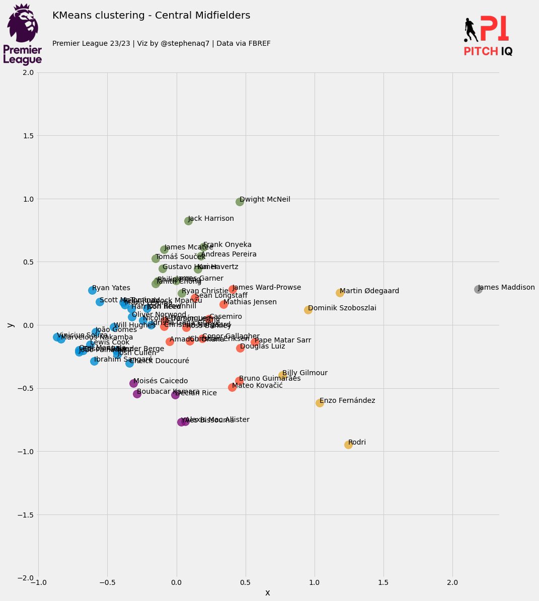
The code below creates a comprehensive visualization of the K-means clustering results, including player positions, cluster assignments, and additional branding elements such as logos and titles. Here’s a breakdown of the code:
- Scatter Plot Creation:
- Generate a scatter plot using Seaborn’s
lmplotfunction. - The plot is based on the x and y coordinates provided in the DataFrame
df. - Data points are colored based on their cluster labels.
- Generate a scatter plot using Seaborn’s
- Adding Player Names to Plot:
- Add player names as annotations to the scatter plot.
- Each annotation is positioned at the corresponding x and y coordinates.
- Adding Title and Logos:
- Set up the main figure and axes for additional elements.
- Add a title indicating the type of clustering and the position.
- Include logos for visual enhancement and branding.
- Set up axes and turn off ticks for the logos.
- Adjusting Plot Properties:
- Set the limits and labels for the x and y axes.
- Adjust tick parameters and font sizes for better readability.
- Display Plot:
- Ensure proper layout and spacing.
- Show the plot with all the added elements.
def create_clustering_chart(df,position):
    # Create the scatter plot using lmplot
    ax = sns.lmplot(x="x", y="y", hue='cluster', data=df, legend=False,
                    fit_reg=False, size=15, scatter_kws={"s": 250})

    texts = []
    for x, y, s in zip(df.x, df.y, df.name):
        texts.append(plt.text(x, y, s,fontweight='light'))


    # Additional axes for logos and titles
    fig = plt.gcf()
    ax1 = plt.gca()

    # Add title and logos to the current figure
    fig.text(.1, 1.08, f'KMeans clustering - {position}', size=20, font='Karla')
    fig.text(.1, 1.03, 'Premier League 23/23 | Viz by @stephenaq7 | Data via FBREF', size=14, font='Karla')

    ax2 = fig.add_axes([0.01, 0.175, 0.07, 1.75])
    ax2.axis('off')
    img = image.imread('/Users/stephenahiabah/Desktop/GitHub/Webs-scarping-for-Fooball-Data-/Images/premier-league-2-logo.png')
    ax2.imshow(img)

    ax3 = fig.add_axes([0.85, 0.175, 0.1, 1.75])
    ax3.axis('off')
    img = image.imread('/Users/stephenahiabah/Desktop/GitHub/Webs-scarping-for-Fooball-Data-/outputs/piqmain.png')
    ax3.imshow(img)

    # Set axis limits and labels for the lmplot
    ax1.set(ylim=(-2, 2))
    plt.tick_params(labelsize=15)
    plt.xlabel("PC 1", fontsize=20)
    plt.ylabel("PC 2", fontsize=20)

    plt.tight_layout()
    plt.show()

create_clustering_chart(kmeans_df,position)
In this plot, each color represents a cluster.
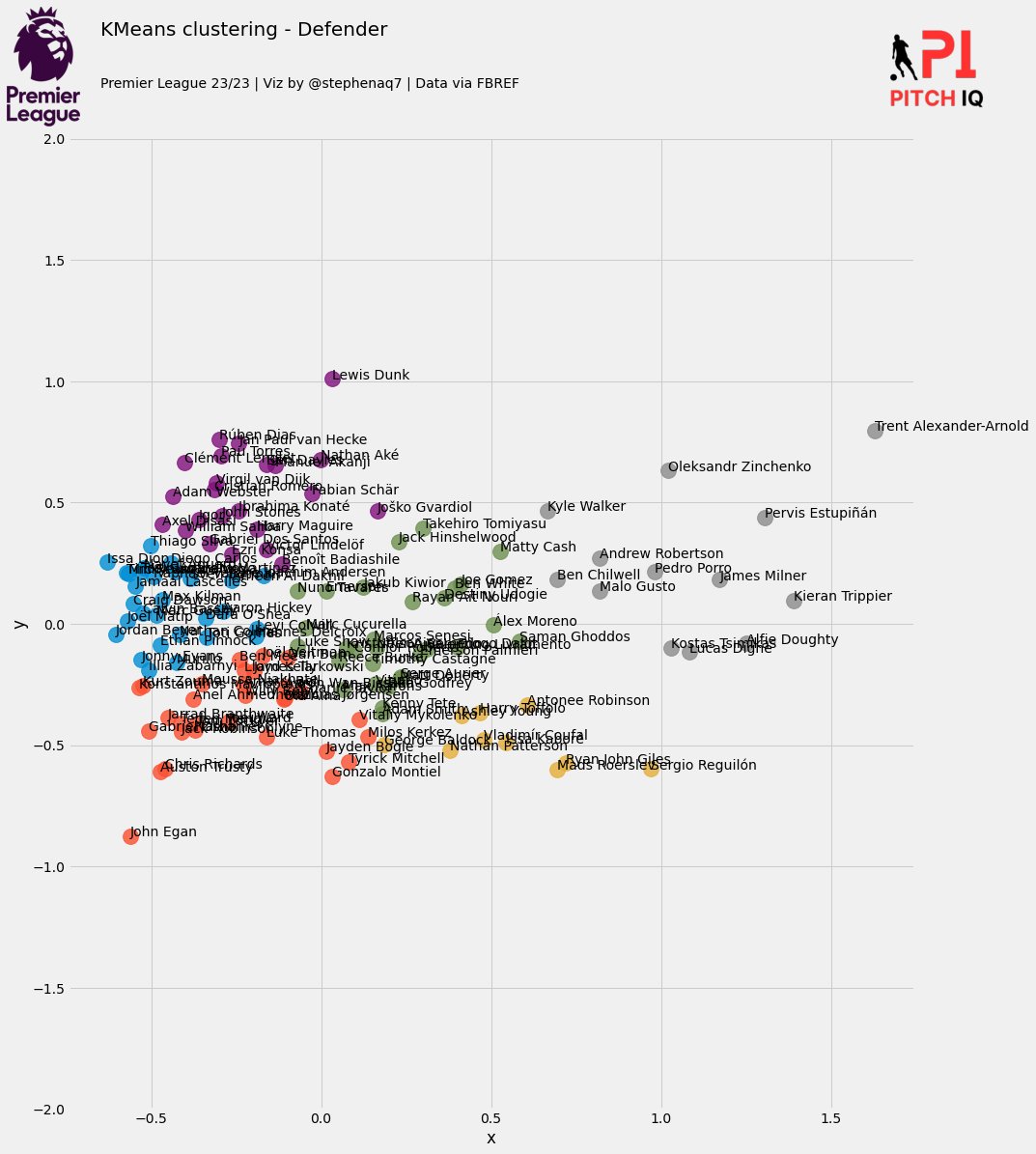
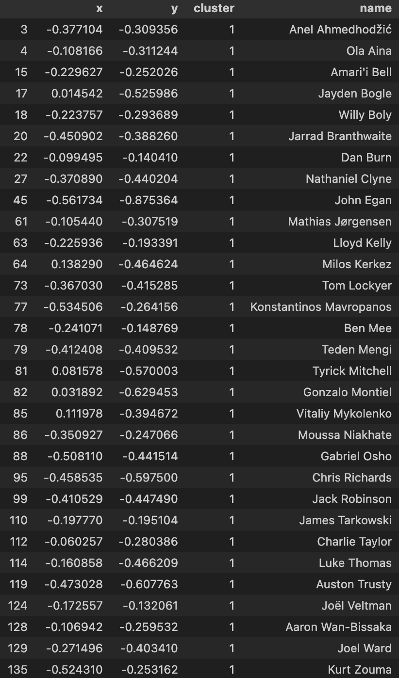
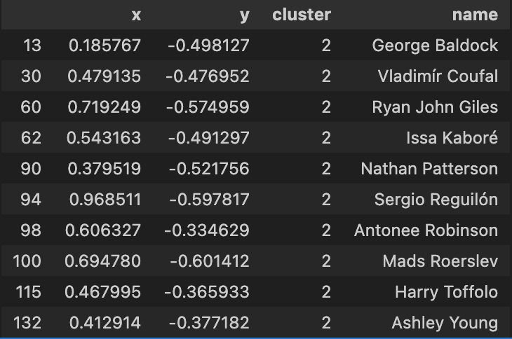
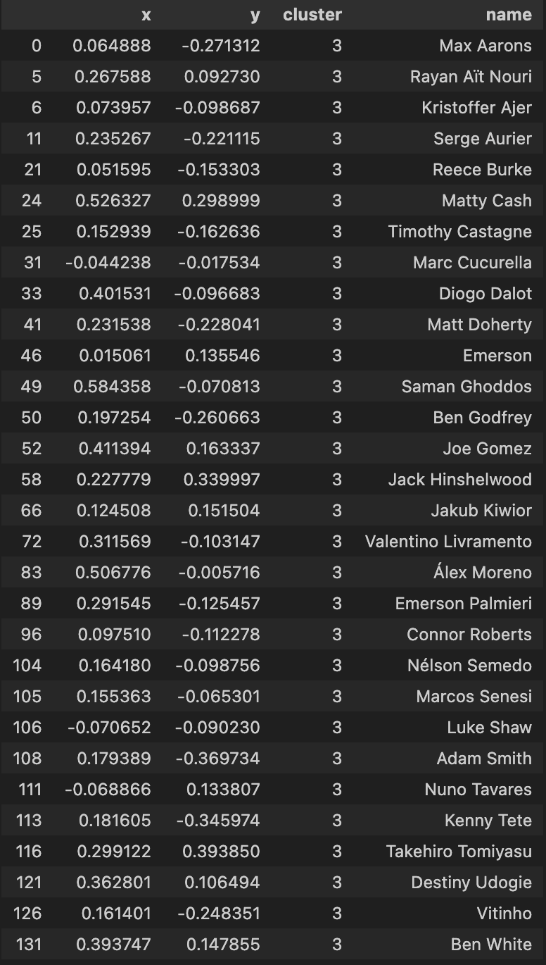
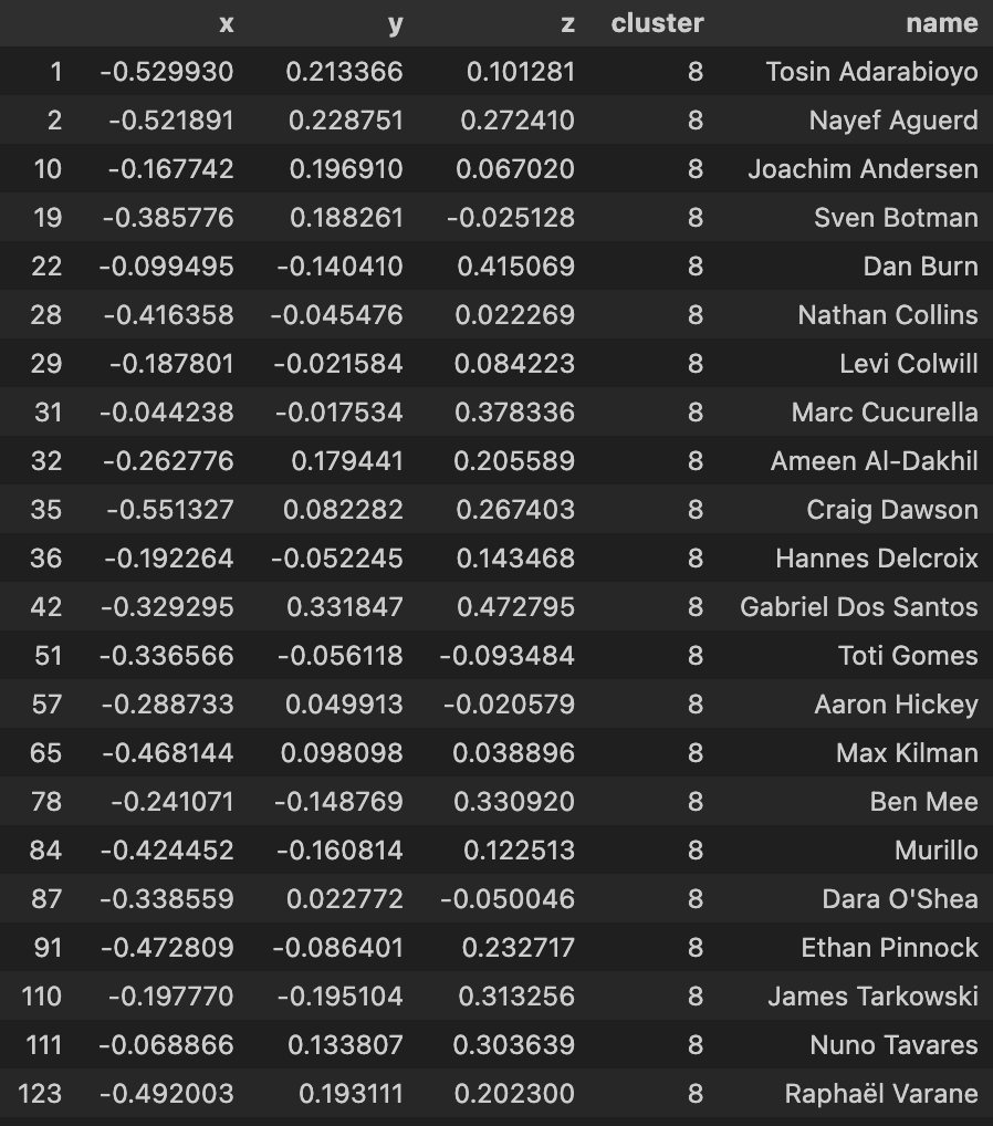
Let’s now inspect what players have been grouped together in each cluster
The following code below will print out the respective dataframe for each cluster:
for i in range(0,6):
    df = kmeans_df[kmeans_df['cluster'] == i]
    print(f'cluster - {i}')
    print(df)
Using my elite ball knowledge :tm: I’ve attempted to ascribe a categorical classing/grouping to each cluster:
| Average Centre Backs | Average Traditional Full Backs |
|---|---|
 |
 |
| Above-Average Defensive Full Backs | Above-Average Attacking Full Backs |
|---|---|
 |
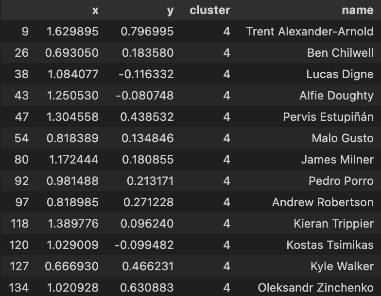 |
| Above-Average Centre Backs |
|---|
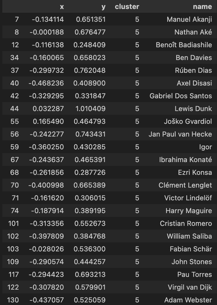 |
In summary, the model seems to be have done a good job in being able to group players together. In my personal opinion, I dont agree with some of the names in the Average Centre Backs and Above-Average Defensive Full Backs cluster but i think its more a question of refining the data that I have applied the PCA algorithm with.
I will spend some more time finding the most appropriate features with a more refined approach to feature selection with a more detailed exploratory data analysis methodology against the web-scraped FBREF data set.
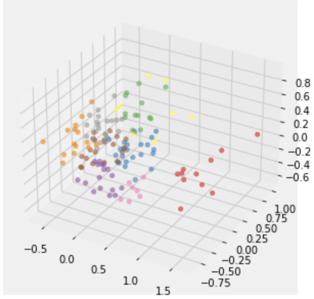
3-D KMeans Analysis
Next, we will create the DataFrame key_stats_df_3d and similarly apply a Principal Component Analysis (PCA) to reduce the dimensions to three. This approach enables us to visualize our players in a three-dimensional space, facilitating the identification of relationships through a comprehensive 3D analysis.
from sklearn import preprocessing

player_names_3d = key_stats_df_3d['Player'].tolist()

df_3d = key_stats_df_3d.drop(['Player'], axis = 1)

x = df_3d.values
scaler = preprocessing.MinMaxScaler()
x_scaled = scaler.fit_transform(x)
X_norm = pd.DataFrame(x_scaled)

from sklearn.decomposition import PCA

pca = PCA(n_components = 3)
df1 = pd.DataFrame(pca.fit_transform(X_norm))

import re, seaborn as sns
from sklearn.cluster import KMeans
from matplotlib import pyplot as plt
from mpl_toolkits.mplot3d import Axes3D
from matplotlib.colors import ListedColormap


%matplotlib inline
df1.columns = ['PC1','PC2', 'PC3']

ax = plt.figure().gca(projection='3d')

ax.scatter(df1['PC1'], df1['PC2'], df1['PC3'], s=40)

plt.show()

wcss = []
for i in range(1, 15):
  kmeans = KMeans(n_clusters = i, init = 'k-means++', random_state = 42)
  kmeans.fit(df1)
  wcss.append(kmeans.inertia_)

plt.plot(range(1, 15), wcss)
plt.xlabel('Number of Clusters (K)')
plt.ylabel('WCSS')
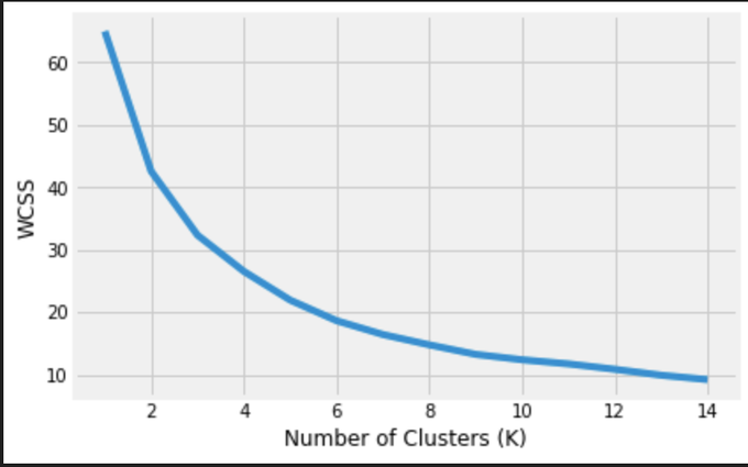
According to the elbow method, we determine that K=9, identified as the point where the rate of decrease in WCSS slows down significantly on our graph.
Now, let’s proceed to train a K-means model for K=9 and observe its performance.
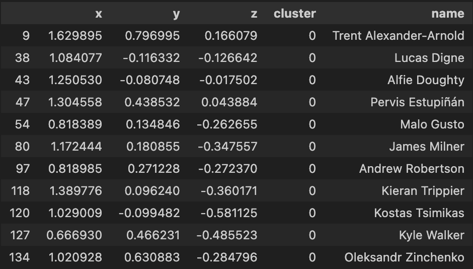
After training and using the trained model, each player in the dataset now has a number from 0 to 8 that represents their set. Let’s put this information in our reduced dataset and then plot it with the results of K-means.
In this plot, each color represents a cluster.
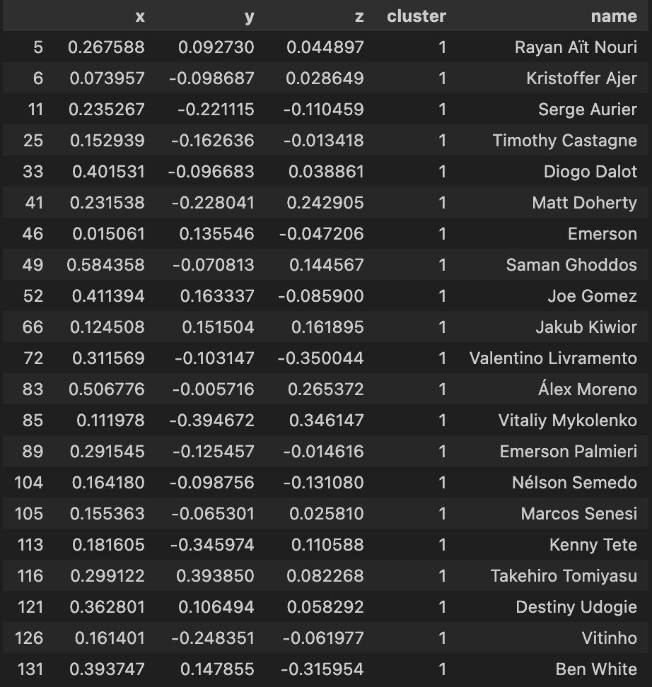
Let’s now inspect what players have been grouped together in each cluster
| Cluster 1 | Cluster 2 |
|---|---|
 |
 |
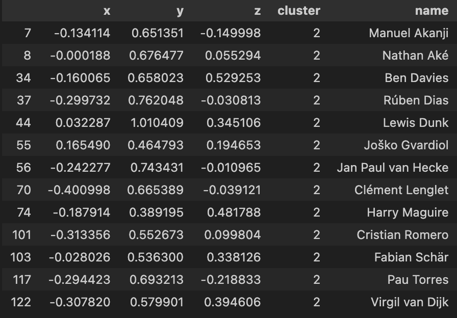
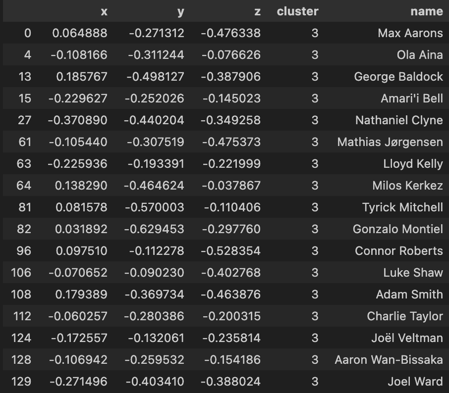
| Cluster 3 | Cluster 4 |
|---|---|
 |
 |
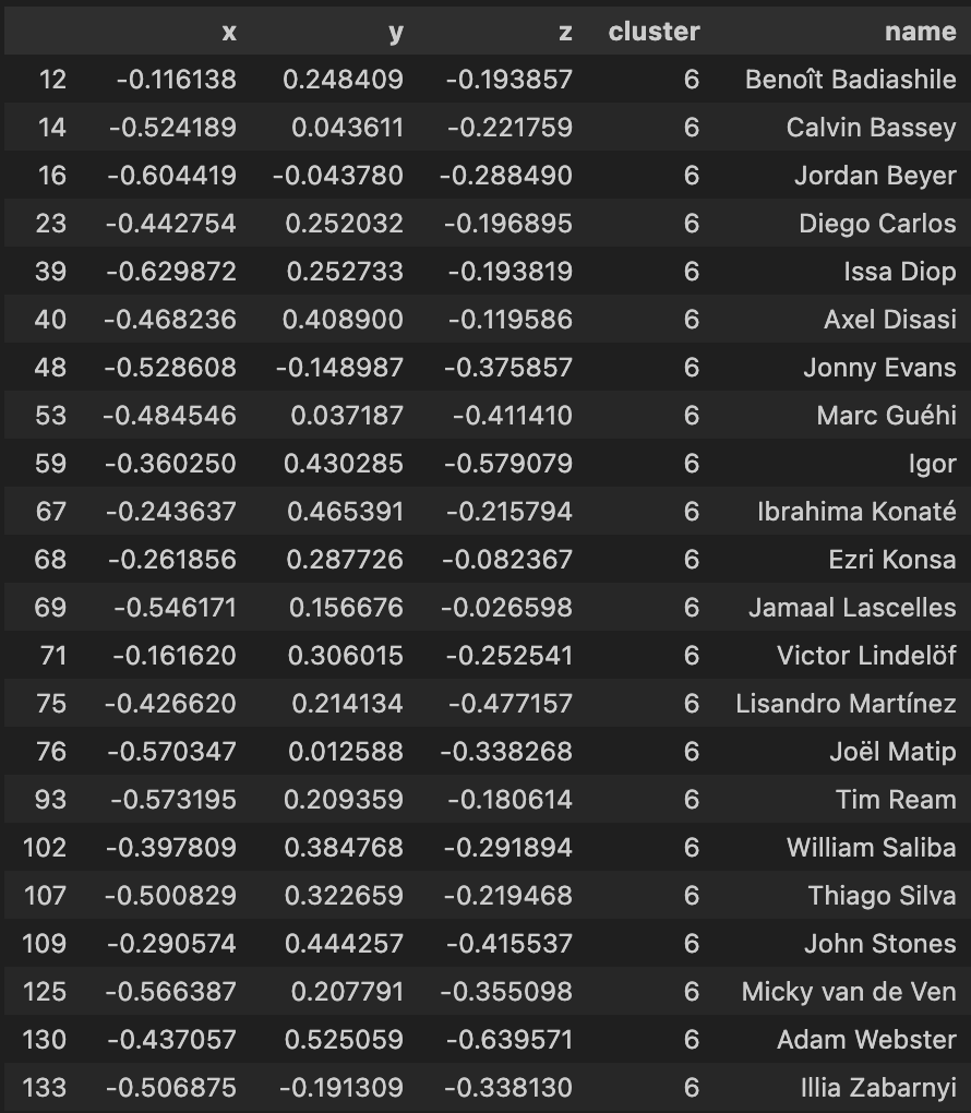
| Cluster 5 | Cluster 6 |
|---|---|
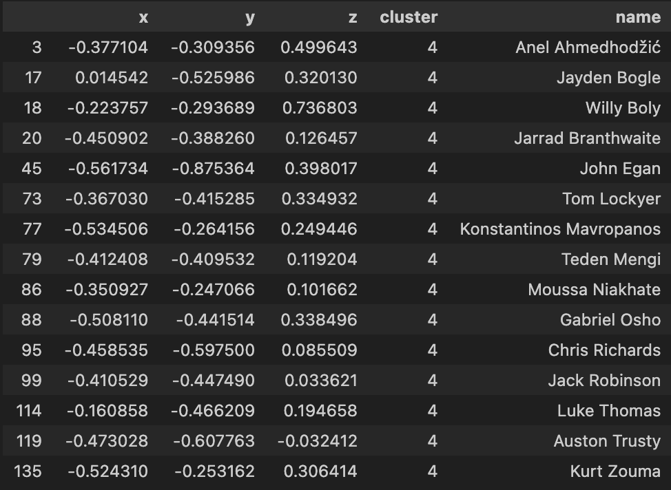 |
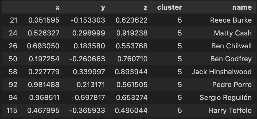 |
| Cluster 7 | Cluster 8 |
|---|---|
 |
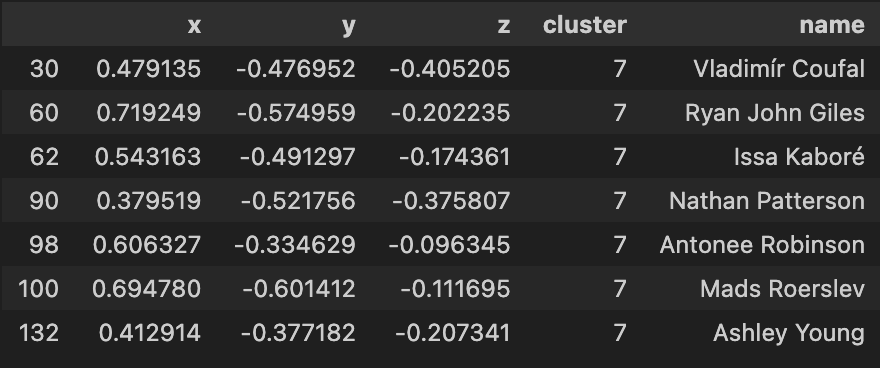 |
| Cluster 9 |
|---|
 |
Using the 3-d KMeans for this dataset overall has been quite hit or miss as you indicate from the clusters above. Again much like the 2d model, I will have to apply a more comprehensive feature selection process to refine these outputs
Conclusion
In conclusion, this post serves as a valuable addition to a series of tutorials aimed at empowering users to utitlizie data science techniques to better understand manipulate data available from FBREF as well as generating insightful data visualizations,and breif introduction into using python libraries such as sk.learn.
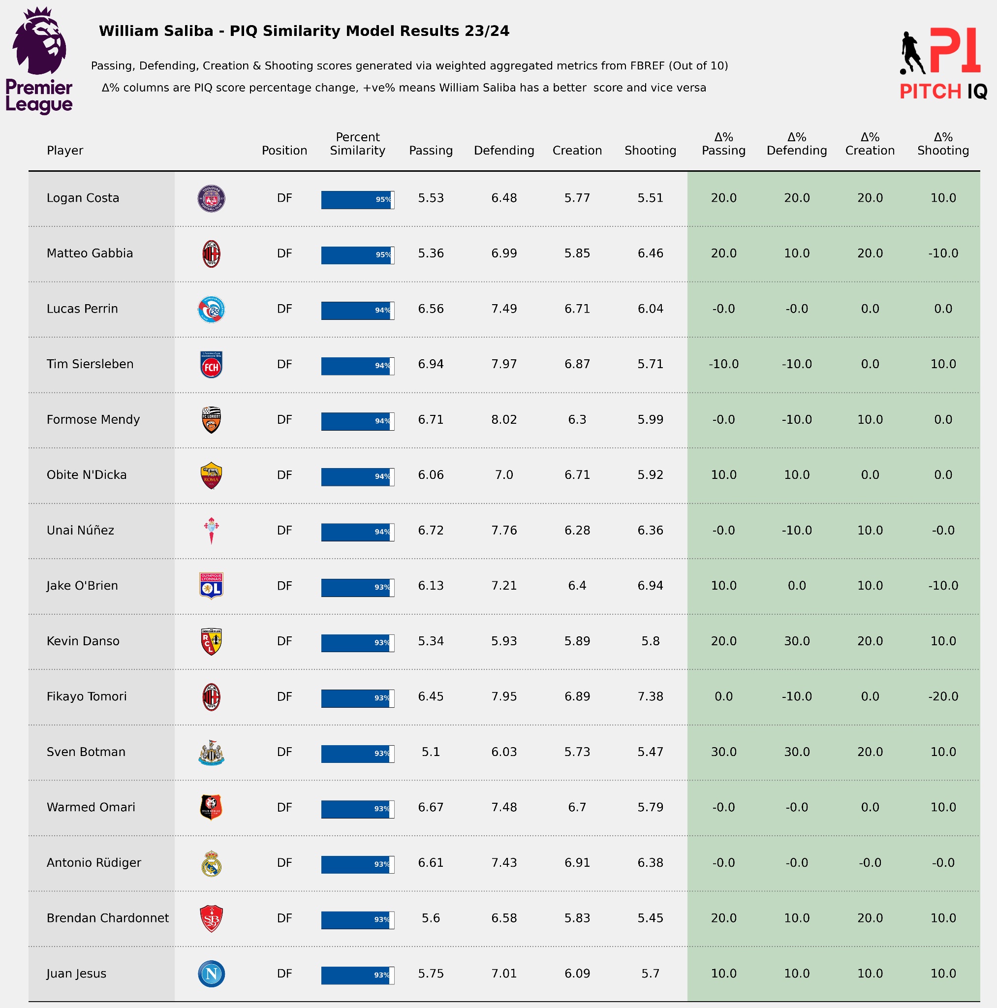
In the next post we’ll be using KMeans clustering to start building a player similarity model
Thanks for reading
Steve

Comments