52 min to read
Figuring Out xG pt2
Advanced analysis of expected goals (xG) in football
In Part 1 of my series of posts on Figuring Out xG, we successfully achieved the following items;
-
Develop efficient functions to aggregate data from FBRef & FotMob.
-
Perform data manipulation tasks to transform raw data into clean, structured datasets suitable for analysis
-
Create data visualizations using the obtained datasets.
-
Evaluate significant metrics that aid in making assertions on team performance.
In Part 2 of our analysis, we will delve into more advanced visualizations, examining xG performance when compared to actual goals scored and conceded.
Applying xG metrics to assess Team Performance
This post by Football Whispers goes in great detail explaining the statiscal significance and implications of using xG to assess how well a team is playing.
In summary this article outlines Expected Goals (xG / xGA) in football, a statistical metric used to assess the likelihood of a shot resulting in a goal. It emphasizes the importance of xG in making accurate predictions for sports betting, especially in scenarios like ante-post bets and short-term success. The article further discusses how xG is calculated, its advantages, and its application in analyzing teams’ performances based on goals scored and conceded. Additionally, it highlights the relevance of xG in understanding player and team effectiveness, offering insights for making informed analyses.
It is therefore key to understand how well teams actually perform in real terms against their xG and xGA with the goals they actually score and conceed.
This post will delve into how to visually represent EPL Teams actual performance vs their statisitcal performance.
In order to capture a teams offensive performance, we will simple calculate goals_for - xg_for and their defensive performance will be goals_against - xg_against.
Setup
The set up remains the same as in Part 1, but as a refresher, please find the key imports and modules below.
import os
import requests
import pandas as pd
from bs4 import BeautifulSoup
import seaborn as sb
import matplotlib.pyplot as plt
import matplotlib as mpl
import warnings
import numpy as np
from math import pi
from urllib.request import urlopen
import matplotlib.patheffects as pe
from highlight_text import fig_text
from adjustText import adjust_text
from tabulate import tabulate
import matplotlib.style as style
import unicodedata
from fuzzywuzzy import fuzz
from fuzzywuzzy import process
import matplotlib.pyplot as plt
import matplotlib.ticker as ticker
import matplotlib.patheffects as path_effects
import matplotlib.font_manager as fm
import matplotlib.colors as mcolors
from matplotlib import cm
from highlight_text import fig_text

from PIL import Image
import urllib
import os
import math
xG vs Actuals
Functions
In Part 1, I outlined a way of pulling a generic dataframe from a webpage in FBREF (shown below), using the function generate_league_data.
def generate_league_data(x):
    url = x
    page = urlopen(url).read()
    soup = BeautifulSoup(page)
    count = 0
    table = soup.find("tbody")

    pre_df = dict()
    features_wanted =  {"team" , "games","wins","draws","losses", "goals_for","goals_against", "points", "xg_for","xg_against","xg_diff","attendance","xg_diff_per90", "last_5"} #add more features here!!
    rows = table.find_all('tr')
    for row in rows:
        for f in features_wanted:
            if (row.find('th', {"scope":"row"}) != None) & (row.find("td",{"data-stat": f}) != None):
                cell = row.find("td",{"data-stat": f})
                a = cell.text.strip().encode()
                text=a.decode("utf-8")
                if f in pre_df:
                    pre_df[f].append(text)
                else:
                    pre_df[f]=[text]

    df = pd.DataFrame.from_dict(pre_df)
    df["games"] = pd.to_numeric(df["games"])
    df["xg_diff_per90"] = pd.to_numeric(df["xg_diff_per90"])
    df["minutes_played"] = df["games"] *90
    return(df)
So will we re-suse this fucntion and assign it to the variable df.
df = generate_league_data("https://fbref.com/en/comps/9/Premier-League-Stats")
Now however we need to perform some manipulations in order to get the offensive and defensive difference figure per team.
Offensive performance will be:
df['goals_for'] = pd.to_numeric(df["goals_for"])
df['xg_for']= pd.to_numeric(df["xg_for"])

df['diff'] = df['goals_for'] - df['xg_for']
df
Offensive performance will be:
df['goals_against'] = pd.to_numeric(df["goals_against"])
df['xg_against']= pd.to_numeric(df["xg_against"])

df['diff_conc'] = df['goals_against'] - df['xg_against']
df
Matplotlib
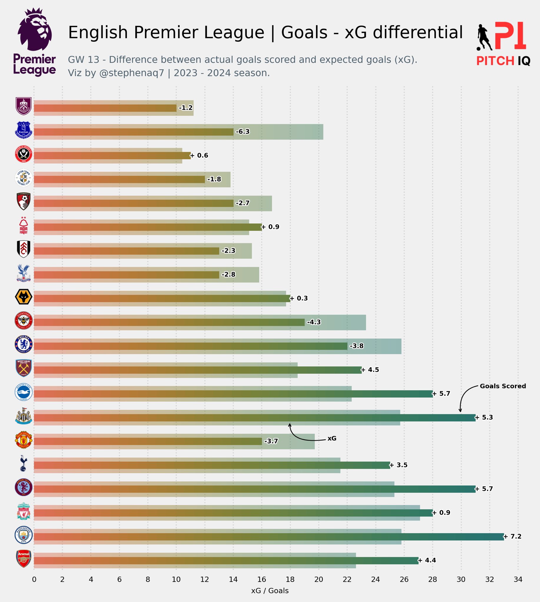
The following code creates a horizontal bar chart using the Matplotlib library in Python. It visualizes the difference between actual goals scored and expected goals (xG) for teams in the English Premier League for a specific game week (GW 13 of the 2023-2024 season). The code also includes additional annotations and logos. Let’s break down the code into steps:
1: Setup the Figure and Axes:
Creates a figure with a specified size and resolution. Adds a subplot to the figure.
fig = plt.figure(figsize=(8, 8), dpi=300)
ax = plt.subplot(111)
2: Customize Axes Properties:
Hides the left spine, removes y-axis ticks, sets x-axis label, adjusts tick label size, and adds a light grey grid.
ax.spines['left'].set_visible(False)
ax.set_yticks([])
ax.xaxis.set_major_locator(ticker.MultipleLocator(2))
ax.xaxis.set_label_text('xG / Goals', size=7)
ax.tick_params(labelsize=7)
ax.grid(axis='x', color='lightgrey', ls=':')
3: Plot xG Bars
Plots horizontal bars representing expected goals (xG) for each team. Uses a colormap (‘SOC’) to add a gradient effect to the bars.
bars_ = ax.barh(df.index, df['xg_for'], height=0.65)
4: Plot Actual Goals Bars:
Plots horizontal bars representing actual goals scored (goals_for) for each team. Uses a colormap (‘SOC’) to add a gradient effect to the bars.
bars_ = ax.barh(df.index, df['goals_for'], height=0.3)
5: Adjust Axes Limits:
Adjusts the x and y-axis limits to accommodate the plotted bars..
ax.set_xlim(-1.85, 35)
ax.set_ylim(-0.5, 20)
6: Add Team Logos and Annotations:
Retrieves team logos from URLs and displays them. Adds text annotations with team names, goal differentials, and other information. Adds text annotations with arrows pointing to specific areas of interest on the plot. Includes a title and additional information about the visualization.
for y in df.index:
    ax_coords = DC_to_NFC((-1.35, y - 0.3))  # Adjusted to prevent overlap
    team_id = df['team_id'].iloc[y]
    team = df['team'].iloc[y].replace(' ', '\n')
    diff_xg = df['diff'].iloc[y]
    xGOT = df['goals_for'].iloc[y]
    if diff_xg > 0:
        text_sign = '+'
    else:
        text_sign = ''
    ax_size = 0.03  # Adjusted size to prevent overlap
    image_ax = fig.add_axes(
        [ax_coords[0], ax_coords[1], ax_size, ax_size],
        fc='None', anchor='C'
    )
    fotmob_url = 'https://images.fotmob.com/image_resources/logo/teamlogo/'
    player_face = Image.open(urllib.request.urlopen(f"{fotmob_url}{team_id}.png"))
    image_ax.imshow(player_face)
    image_ax.axis('off')
When we put it all together, the full code should look like the following.
fig = plt.figure(figsize=(8, 8), dpi=300)
ax = plt.subplot(111)

ax.spines['left'].set_visible(False)
ax.set_yticks([])
ax.xaxis.set_major_locator(ticker.MultipleLocator(2))
ax.xaxis.set_label_text('xG / Goals', size=7)
ax.tick_params(labelsize=7)
ax.grid(axis='x', color='lightgrey', ls=':')

# xG
bars_ = ax.barh(df.index, df['xg_for'], height=0.65)
for bar in bars_:
    bar.set_zorder(1)
    bar.set_facecolor('none')
    x, y = bar.get_xy()
    w, h = bar.get_width(), bar.get_height()
    grad = np.atleast_2d(np.linspace(0, 1 * w / max(df['xg_for']), 256))
    ax.imshow(
        grad, extent=[x, x + w, y, y + h],
        aspect='auto', zorder=3,
        norm=NoNorm(vmin=0, vmax=1), cmap='SOC', alpha=0.45
    )

# Actual Goals Scored
bars_ = ax.barh(df.index, df['goals_for'], height=0.3)
lim = ax.get_xlim() + ax.get_ylim()
for bar in bars_:
    bar.set_zorder(1)
    bar.set_facecolor('none')
    x, y = bar.get_xy()
    w, h = bar.get_width(), bar.get_height()
    grad = np.atleast_2d(np.linspace(0, 1 * w / max(df['goals_for']), 256))
    ax.imshow(
        grad, extent=[x, x + w, y, y + h],
        aspect='auto', zorder=3,
        norm=NoNorm(vmin=0, vmax=1), cmap='SOC'
    )

ax.set_xlim(-1.85, 35)  # Adjusted to accommodate 19 bars
ax.set_ylim(-0.5, 20)  # Adjusted to accommodate 19 bars

DC_to_FC = ax.transData.transform
FC_to_NFC = fig.transFigure.inverted().transform
# -- Take data coordinates and transform them to normalized figure coordinates
DC_to_NFC = lambda x: FC_to_NFC(DC_to_FC(x))
for y in df.index:
    ax_coords = DC_to_NFC((-1.35, y - 0.3))  # Adjusted to prevent overlap
    team_id = df['team_id'].iloc[y]
    team = df['team'].iloc[y].replace(' ', '\n')
    diff_xg = df['diff'].iloc[y]
    xGOT = df['goals_for'].iloc[y]
    if diff_xg > 0:
        text_sign = '+'
    else:
        text_sign = ''
    ax_size = 0.03  # Adjusted size to prevent overlap
    image_ax = fig.add_axes(
        [ax_coords[0], ax_coords[1], ax_size, ax_size],
        fc='None', anchor='C'
    )
    fotmob_url = 'https://images.fotmob.com/image_resources/logo/teamlogo/'
    player_face = Image.open(urllib.request.urlopen(f"{fotmob_url}{team_id}.png"))
    image_ax.imshow(player_face)
    image_ax.axis('off')
    # ax.annotate(
    #     xy=(-1.1, y - 0.32),
    #     text=team,
    #     size=5,
    #     ha='center',
    #     va='center'
    # )
    text_ = ax.annotate(
        xy=(xGOT, y),
        xytext=(8, 0),
        text=f'{text_sign} {diff_xg:.1f}',
        size=6,
        ha='center',
        va='center',
        textcoords='offset points',
        weight='bold'
    )
    text_.set_path_effects(
        [path_effects.Stroke(linewidth=1.5, foreground='white'), path_effects.Normal()]
    )
text_ = ax.annotate(
    xy=(30, 6),
    xytext=(40,30),
    text='Goals Scored',
    size=6,
    ha='center',
    va='center',
    textcoords='offset points',
    weight='bold',
    arrowprops=dict(
            arrowstyle="->", shrinkA=0, shrinkB=5, color="black", linewidth=0.75,
            connectionstyle="angle3,angleA=-10,angleB=100"
    )
)

text_ = ax.annotate(
    xy=(18, 6),
    xytext=(40,-20),
    text='xG',
    size=6,
    ha='center',
    va='center',
    textcoords='offset points',
    weight='bold',
    arrowprops=dict(
            arrowstyle="->", shrinkA=0, shrinkB=5, color="black", linewidth=0.75,
            connectionstyle="angle3,angleA=10,angleB=-100"
    )
)

fig_text(
    x=0.18, y=0.95,
    s="English Premier League | Goals - xG differential",
    va='bottom', ha='left',
    fontsize=16, color='black', font='Karla',
)
fig_text(
    x=0.18, y=0.89,
    s="GW 13 - Difference between actual goals scored and expected goals (xG).\nViz by @stephenaq7 | 2023 - 2024 season.",
    va='bottom', ha='left',
    fontsize=9, color='#4E616C', font='Karla'
)

ax2 = fig.add_axes([0.09, 0.075, 0.07, 1.75])
ax2.axis('off')
img = image.imread('/Users/stephenahiabah/Desktop/GitHub/Webs-scarping-for-Fooball-Data-/Images/premier-league-2-logo.png')
ax2.imshow(img)


### Add Stats by Steve logo
ax3 = fig.add_axes([0.85, 0.075, 0.1, 1.75])
ax3.axis('off')
img = image.imread('/Users/stephenahiabah/Desktop/GitHub/Webs-scarping-for-Fooball-Data-/outputs/piqmain.png')
ax3.imshow(img)


plt.show()  # Added this line to display the plot
Our final visual should look as follows:
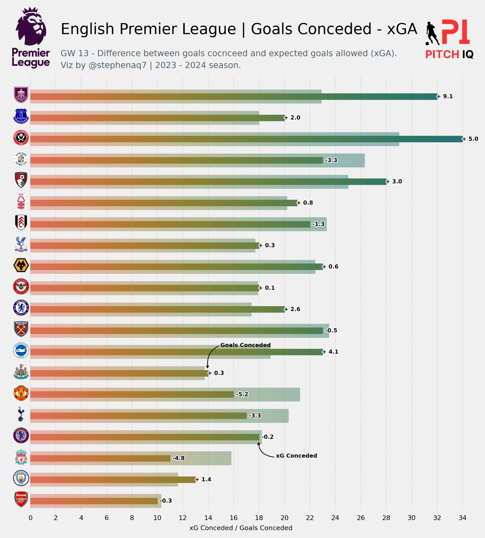
Using the same structure and principles we can simple change the variables we’re plotting to now be the defensive performance metrics. The full code for that can be found below.
fig = plt.figure(figsize=(8, 8), dpi=300)
ax = plt.subplot(111)

ax.spines['left'].set_visible(False)
ax.set_yticks([])
ax.xaxis.set_major_locator(ticker.MultipleLocator(2))
ax.xaxis.set_label_text('xG Conceded / Goals Conceded', size=7)
ax.tick_params(labelsize=7)
ax.grid(axis='x', color='lightgrey', ls=':')

# xG Against
bars_ = ax.barh(df.index, df['xg_against'], height=0.65)
for bar in bars_:
    bar.set_zorder(1)
    bar.set_facecolor('none')
    x, y = bar.get_xy()
    w, h = bar.get_width(), bar.get_height()
    grad = np.atleast_2d(np.linspace(0, 1 * w / max(df['xg_for']), 256))
    ax.imshow(
        grad, extent=[x, x + w, y, y + h],
        aspect='auto', zorder=3,
        norm=NoNorm(vmin=0, vmax=1), cmap='SOC', alpha=0.45
    )

# Actual Goals Conceded
bars_ = ax.barh(df.index, df['goals_against'], height=0.3)
lim = ax.get_xlim() + ax.get_ylim()
for bar in bars_:
    bar.set_zorder(1)
    bar.set_facecolor('none')
    x, y = bar.get_xy()
    w, h = bar.get_width(), bar.get_height()
    grad = np.atleast_2d(np.linspace(0, 1 * w / max(df['goals_against']), 256))
    ax.imshow(
        grad, extent=[x, x + w, y, y + h],
        aspect='auto', zorder=3,
        norm=NoNorm(vmin=0, vmax=1), cmap='SOC'
    )

ax.set_xlim(-1.85, 35)  # Adjusted to accommodate 19 bars
ax.set_ylim(-0.5, 20)  # Adjusted to accommodate 19 bars

DC_to_FC = ax.transData.transform
FC_to_NFC = fig.transFigure.inverted().transform
# -- Take data coordinates and transform them to normalized figure coordinates
DC_to_NFC = lambda x: FC_to_NFC(DC_to_FC(x))
for y in df.index:
    ax_coords = DC_to_NFC((-1.35, y - 0.3))  # Adjusted to prevent overlap
    team_id = df['team_id'].iloc[y]
    team = df['team'].iloc[y].replace(' ', '\n')
    diff_xg = df['diff_conc'].iloc[y]
    xGOT = df['goals_against'].iloc[y]
    if diff_xg > 0:
        text_sign = '+'
    else:
        text_sign = ''
    ax_size = 0.03  # Adjusted size to prevent overlap
    image_ax = fig.add_axes(
        [ax_coords[0], ax_coords[1], ax_size, ax_size],
        fc='None', anchor='C'
    )
    fotmob_url = 'https://images.fotmob.com/image_resources/logo/teamlogo/'
    player_face = Image.open(urllib.request.urlopen(f"{fotmob_url}{team_id}.png"))
    image_ax.imshow(player_face)
    image_ax.axis('off')
    # ax.annotate(
    #     xy=(-1.1, y - 0.32),
    #     text=team,
    #     size=5,
    #     ha='center',
    #     va='center'
    # )
    text_ = ax.annotate(
        xy=(xGOT, y),
        xytext=(8, 0),
        text=f'{text_sign} {diff_xg:.1f}',
        size=6,
        ha='center',
        va='center',
        textcoords='offset points',
        weight='bold'
    )
    text_.set_path_effects(
        [path_effects.Stroke(linewidth=1.5, foreground='white'), path_effects.Normal()]
    )
text_ = ax.annotate(
    xy=(14, 6),
    xytext=(40,30),
    text='Goals Conceded',
    size=6,
    ha='center',
    va='center',
    textcoords='offset points',
    weight='bold',
    arrowprops=dict(
            arrowstyle="->", shrinkA=0, shrinkB=5, color="black", linewidth=0.75,
            connectionstyle="angle3,angleA=-10,angleB=100"
    )
)

text_ = ax.annotate(
    xy=(18, 3),
    xytext=(40,-20),
    text='xG Conceded',
    size=6,
    ha='center',
    va='center',
    textcoords='offset points',
    weight='bold',
    arrowprops=dict(
            arrowstyle="->", shrinkA=0, shrinkB=5, color="black", linewidth=0.75,
            connectionstyle="angle3,angleA=10,angleB=-100"
    )
)
fig_text(
    x=0.18, y=0.95,
    s="English Premier League | Goals Conceded - xGA",
    va='bottom', ha='left',
    fontsize=16, color='black', font='Karla',
)
fig_text(
    x=0.18, y=0.89,
    s="GW 13 - Difference between goals cocnceed and expected goals allowed (xGA).\nViz by @stephenaq7 | 2023 - 2024 season.",
    va='bottom', ha='left',
    fontsize=9, color='#4E616C', font='Karla'
)

ax2 = fig.add_axes([0.09, 0.075, 0.07, 1.75])
ax2.axis('off')
img = image.imread('/Users/stephenahiabah/Desktop/GitHub/Webs-scarping-for-Fooball-Data-/Images/premier-league-2-logo.png')
ax2.imshow(img)


### Add Stats by Steve logo
ax3 = fig.add_axes([0.85, 0.075, 0.1, 1.75])
ax3.axis('off')
img = image.imread('/Users/stephenahiabah/Desktop/GitHub/Webs-scarping-for-Fooball-Data-/outputs/piqmain.png')
ax3.imshow(img)


plt.show()  # Added this line to display the plot
Our final visual should look as follows:
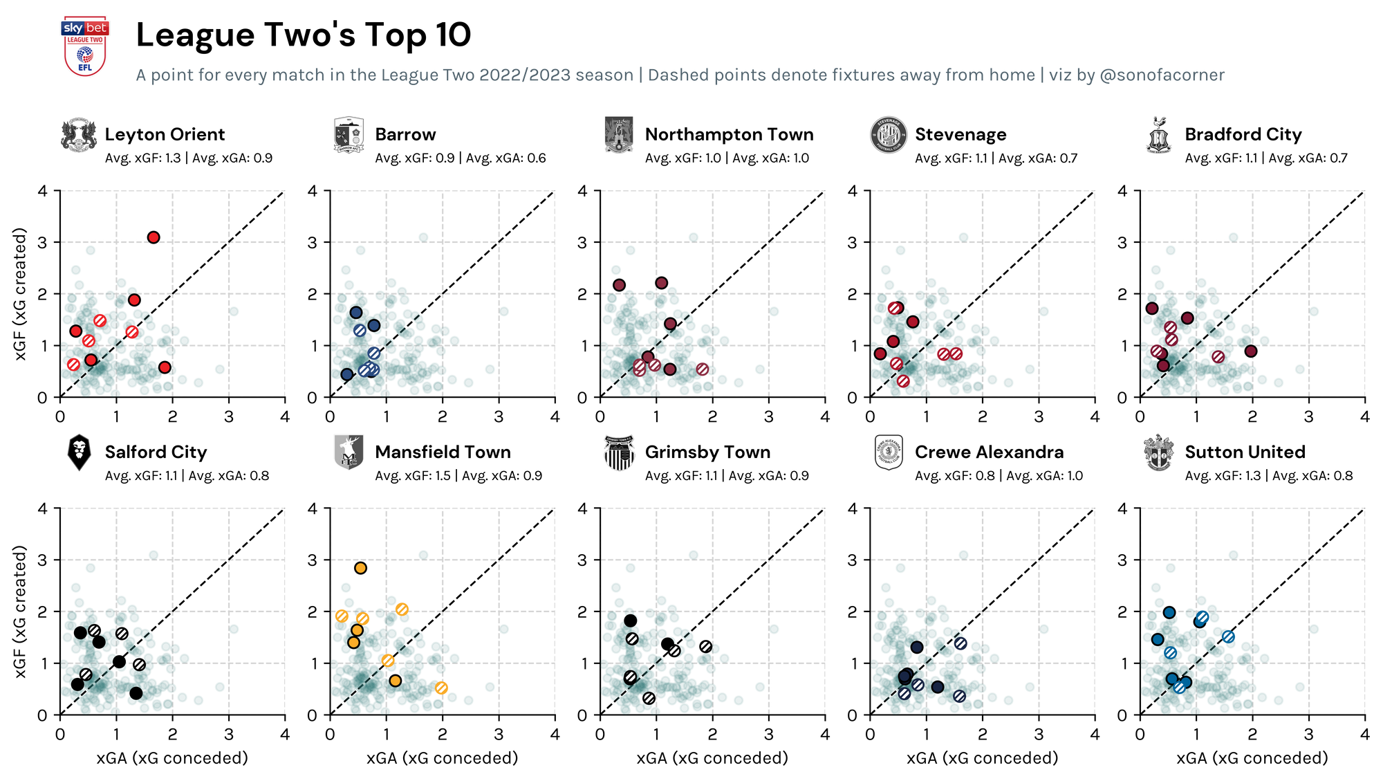
xG Scatter Plots
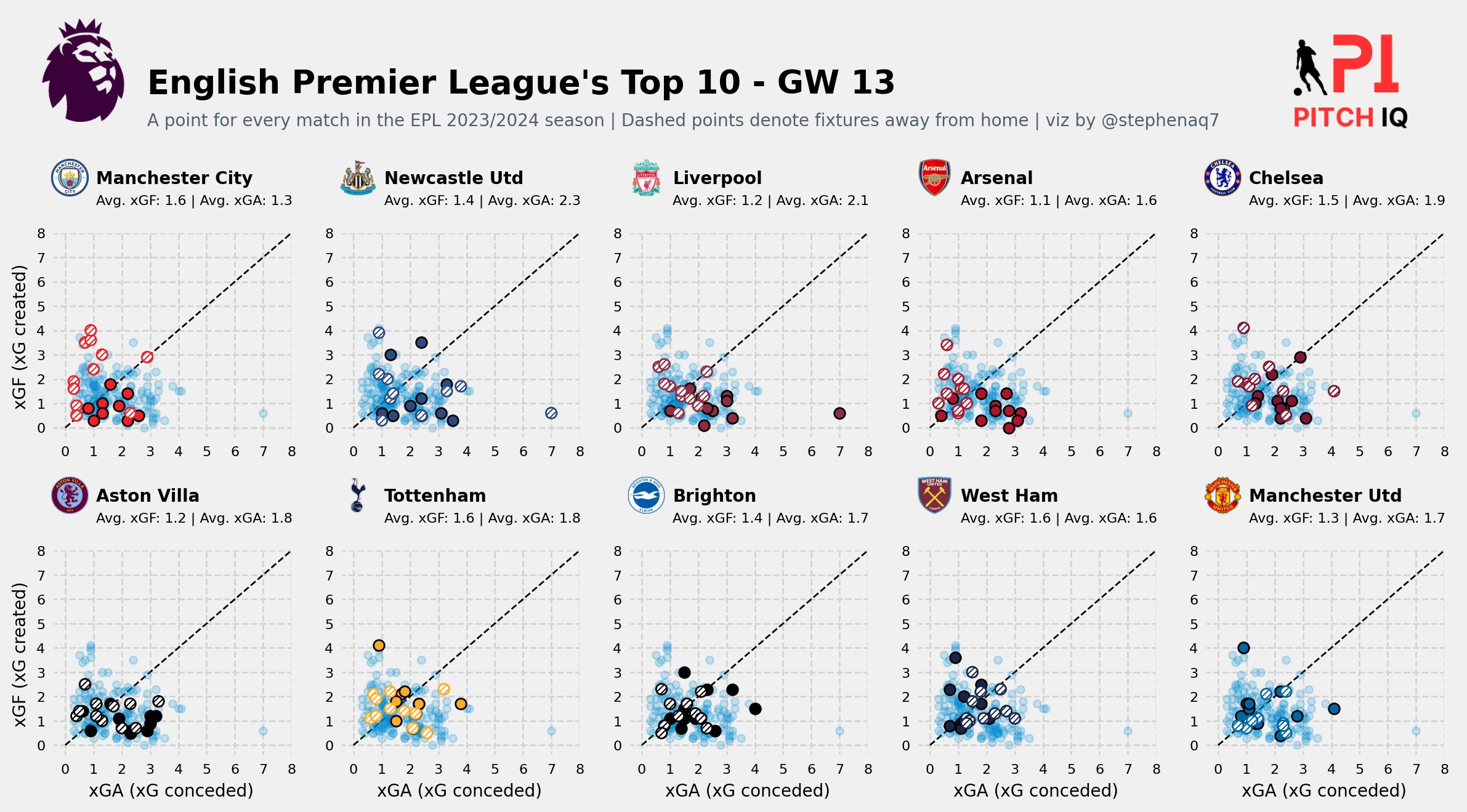
We’ll now move on to creating the final visual for this series of posts; xG Scatter plots.
The xG scatter chart provides a comprehensive visual representation of a football team’s performance in terms of expected goals, allowing analysts and enthusiasts to assess how well a team is performing in attack and defense and identify patterns or anomalies in their gameplay.
The purpose of creating an xG (Expected Goals) scatter chart is to visually represent and analyze the performance of a football team in terms of both conceding and scoring goals, based on expected goals metrics.
Here’s a breakdown of the key aspects and insights that can be gained from an xG scatter chart
xG Conceded (xGA):- The
x-axistypically represents the expected goals conceded by a team (xGA). Each point on thex-axiscorresponds to a specific match or event. - Points to the right of the
y-axisindicate matches where the team’s defensive performance was better than the expected goals model predicted.
- The
xG Created (xGF):- The
y-axisrepresents the expected goals created by a team (xGF). Each point on they-axiscorresponds to the same matches or events as thex-axis. - Points above the
x-axisindicate matches where the team created more goal-scoring opportunities than the expected goals model predicted.
- The
Scatter Points:- Each point in the
scatter chartrepresents a specific match or event for the team. - Points closer to the origin (
0,0) suggest that the team performed close to the expectations in terms of goals conceded and created.
- Each point in the
Differentiating Home and Away Matches:- The
scatter chartoften uses different markers or colors to distinguish betweenhomeandawaymatches. - For example, points for
homematches might be represented by filled circles, while points forawaymatches could be represented by hatched circles.
- The
Analysis of Outliers:Outliers, points that deviate significantly from the main cluster, can be analyzed to identify exceptional performances or deviations from expected outcomes.- For instance, points in the upper-left quadrant (low
xGFand lowxGA) might represent matches where the team underperformed in terms of both attacking and defending.
Reference Line:- The diagonal dashed line from the bottom-left to the top-right represents a
reference linewherexGAis equal toxGF. Points above this line suggest matches where the team created more goal-scoring opportunities than they conceded.
- The diagonal dashed line from the bottom-left to the top-right represents a
Data Prepartion & Manipulation
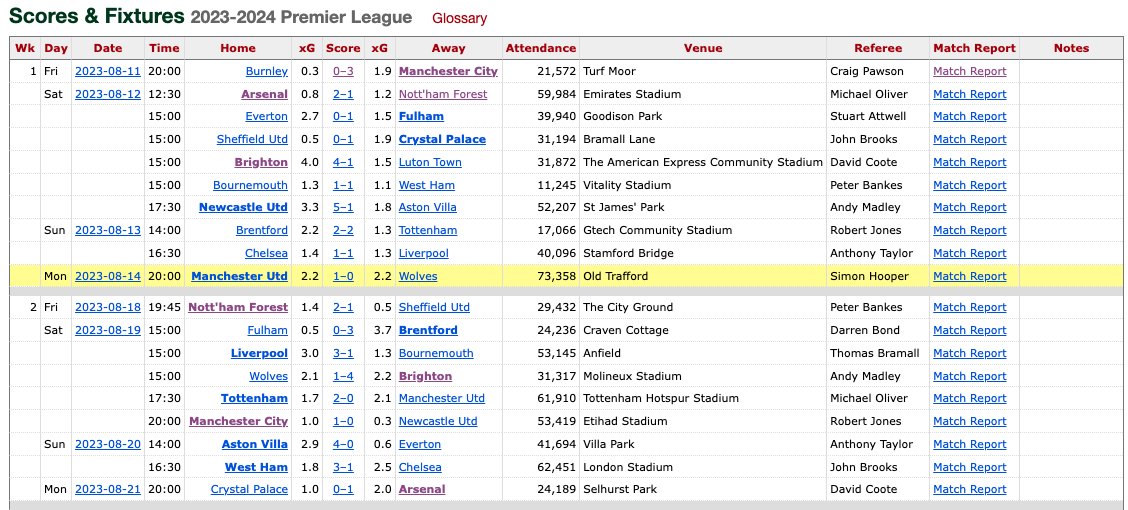
For this visual, we’ll be using another subpage from FBREF. This page has all the recent scores and upcoming fixtures in the EPL. A snippet of the page is shown below.
The following code is a Python script for web scraping football fixtures data from a specific URL using the requests library to fetch the HTML content and BeautifulSoup from the bs4 (Beautiful Soup) library to parse the HTML and extract information. Additionally, it uses the pandas library to read the HTML tables into a DataFrame.
We’ll call our dataframe fixtures.
url = 'https://fbref.com/en/comps/9/schedule/Premier-League-Scores-and-Fixtures'
page =requests.get(url)
soup = BeautifulSoup(page.content, 'html.parser')
html_content = requests.get(url).text.replace('<!--', '').replace('-->', '')
df = pd.read_html(html_content)
fixtures = df[0]
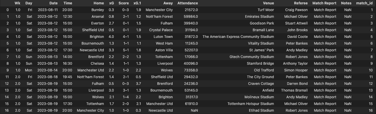
These lines of code clean the fixtures DataFrame by removing rows where the ‘Referee’ column has missing values and then add a new column 'match_id' with unique identifiers for each row in the fixtures DataFrame.
fixtures.dropna(subset=['Referee'], inplace=True)
fixtures['match_id'] = range(1, len(fixtures) + 1)
The resulting table should look like the following:
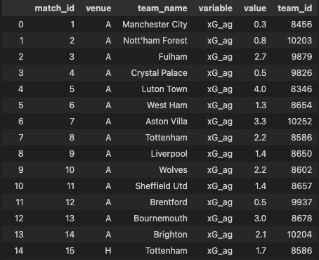
In order to get the data from the fixtures DataFrame in the correct shape to create our visual, we’ll need to do some major surgery to it.
A_fixtures = fixtures.copy()
H_fixtures = fixtures.copy()

A_fixtures['Venue'] = A_fixtures.apply(lambda row: 'A' if row['Away'] == row['Venue'] else 'H', axis=1)

# Create a new column 'team_name' based on 'Home' and 'Away' columns
A_fixtures['team'] = A_fixtures.apply(lambda row: row['Home'] if row['Venue'] == 'H' else row['Away'], axis=1)

# Reshape the DataFrame based on 'match_id'
A_melted_df = A_fixtures.melt(id_vars=['match_id', 'Venue', 'team'], value_vars=['xG', 'xG.1'],
                    var_name='variable', value_name='value')

# Rename the columns as needed
A_melted_df.rename(columns={'Venue': 'venue_code'}, inplace=True)

A_melted_df['variable'] = A_melted_df['variable'].replace({'xG':'xG_ag', 'xG.1': 'xG_for' })


A_Final_df = A_melted_df.merge(fm_ids, on='team', how='left')

A_Final_df.rename(columns={'team': 'team_name'}, inplace=True)

A_Final_df.rename(columns={'venue_code': 'venue'}, inplace=True)


H_fixtures['Venue'] = H_fixtures.apply(lambda row: 'H' if row['Home'] == row['Venue'] else 'A', axis=1)

# Create a new column 'team_name' based on 'Home' and 'Away' columns
H_fixtures['team'] = H_fixtures.apply(lambda row: row['Home'] if row['Venue'] == 'H' else row['Away'], axis=1)

# Reshape the DataFrame based on 'match_id'
H_melted_df = H_fixtures.melt(id_vars=['match_id', 'Venue', 'team'], value_vars=['xG', 'xG.1'],
                    var_name='variable', value_name='value')

# Rename the columns as needed
H_melted_df.rename(columns={'Venue': 'venue_code'}, inplace=True)

H_melted_df['variable'] = H_melted_df['variable'].replace({'xG':'xG_ag', 'xG.1': 'xG_for' })


H_Final_df = H_melted_df.merge(fm_ids, on='team', how='left')

H_Final_df.rename(columns={'team': 'team_name'}, inplace=True)

H_Final_df.rename(columns={'venue_code': 'venue'}, inplace=True)

df = pd.concat([A_Final_df, H_Final_df]).reset_index()
This code snippet appears to be preprocessing football fixtures data, creating two separate DataFrames (A_fixtures and H_fixtures) to represent matches from the perspective of the away and home teams, respectively. The goal is to reshape the data for further analysis. Here’s a step-by-step explanation:
Part 1: Processing Away Fixtures (A_fixtures)
1: A_fixtures = fixtures.copy():
- Creates a copy of the original
fixturesDataFrame, storing it asA_fixtures.
2: A_fixtures['Venue'] = A_fixtures.apply(lambda row: 'A' if row['Away'] == row['Venue'] else 'H', axis=1):
- Adds a new column ‘Venue’ to
A_fixturesbased on the condition: if the ‘Away’ team is equal to the ‘Venue’, set ‘A’; otherwise, set ‘H’.
3: A_fixtures['team'] = A_fixtures.apply(lambda row: row['Home'] if row['Venue'] == 'H' else row['Away'], axis=1):
- Creates a new column ‘team’ in
A_fixturesbased on whether the match is home or away.
4: Reshaping the DataFrame:
A_melted_df = A_fixtures.melt(id_vars=['match_id', 'Venue', 'team'], value_vars=['xG', 'xG.1'], var_name='variable', value_name='value'):- Reshapes the DataFrame based on ‘match_id’, ‘Venue’, ‘team’, and the ‘xG’ and ‘xG.1’ columns.
5: Column Renaming and Transformation:
A_melted_df.rename(columns={'Venue': 'venue_code'}, inplace=True):- Renames the ‘Venue’ column to ‘venue_code’.
A_melted_df['variable'] = A_melted_df['variable'].replace({'xG':'xG_ag', 'xG.1': 'xG_for' }):- Renames the ‘xG’ and ‘xG.1’ columns to ‘xG_ag’ and ‘xG_for’, respectively.
A_Final_df = A_melted_df.merge(fm_ids, on='team', how='left'):- Merges the DataFrame with additional football-related information (
fm_ids) based on the ‘team’ column.
- Merges the DataFrame with additional football-related information (
Part 2: Processing Home Fixtures (H_fixtures)
1: H_fixtures = fixtures.copy():
- Creates a copy of the original
fixturesDataFrame, storing it asH_fixtures.
2: H_fixtures['Venue'] = H_fixtures.apply(lambda row: 'H' if row['Home'] == row['Venue'] else 'A', axis=1):
- Adds a new column ‘Venue’ to
H_fixturesbased on whether the match is home or away.
3: H_fixtures['team'] = H_fixtures.apply(lambda row: row['Home'] if row['Venue'] == 'H' else row['Away'], axis=1):
- Creates a new column ‘team’ in
H_fixturesbased on whether the match is home or away.
4: Reshaping the DataFrame:
H_melted_df = H_fixtures.melt(id_vars=['match_id', 'Venue', 'team'], value_vars=['xG', 'xG.1'], var_name='variable', value_name='value'):- Reshapes the DataFrame based on ‘match_id’, ‘Venue’, ‘team’, and the ‘xG’ and ‘xG.1’ columns.
5: Column Renaming and Transformation:
H_melted_df.rename(columns={'Venue': 'venue_code'}, inplace=True):- Renames the ‘Venue’ column to ‘venue_code’.
H_melted_df['variable'] = H_melted_df['variable'].replace({'xG':'xG_ag', 'xG.1': 'xG_for' }):- Renames the ‘xG’ and ‘xG.1’ columns to ‘xG_ag’ and ‘xG_for’, respectively.
H_Final_df = H_melted_df.merge(fm_ids, on='team', how='left'):- Merges the DataFrame with additional football-related information (
fm_ids) based on the ‘team’ column.
- Merges the DataFrame with additional football-related information (
Combining Away and Home DataFrames (df)
df = pd.concat([A_Final_df, H_Final_df]).reset_index():- Concatenates the
A_Final_dfandH_Final_dfDataFrames vertically to create a combined DataFrame,df. - The
reset_index()method is used to reindex the resulting DataFrame.
- Concatenates the
In summary, this code segment is designed to transform and reshape football fixtures data, separating it into home and away perspectives, and then combining the processed information into a single DataFrame (df). The data is organized for further analysis, potentially involving expected goals (‘xG’) for and against different teams in various match venues.
Our fixtures DataFrame now should have the following shape:
We want to pull out the data and create the chart for the top 10 team in the EPL
top_10 = [
    8456, 10261, 8650, 9825, 8455,
    10252, 8586, 10204, 8654, 10260
]
top_10_colors=[
    '#ed2227', '#2a4b80', '#8c2d42', '#ac152a',
    '#7f1734', '#000000', '#faac28', '#000000',
    '#182544', '#00669d'
]
top_10:- Contains the FotMob IDs of the teams that are in the top 10 of the EPL as of 23/11/23.
top_10_colors:- Contains ten color codes represented as hexadecimal values (e.g.,
'#ed2227'). - Each color code corresponds to an item in the
top_10list. The colors are associated with specific elements, creating a color scheme for the corresponding identifiers in thetop_10list.
- Contains ten color codes represented as hexadecimal values (e.g.,
These lists can be used, for example, to assign distinct colors to specific items in a visual representation, like a bar chart or a plot, where each value in top_10 is associated with a particular color in top_10_colors.
Matplotlib
Before we can plot a multi-chart plot, we need to create a function to plot the data for each induvidual team.
This code defines a Python function plot_scatter_xg that is designed to create a scatter plot representing the expected goals (xG) for and against a specific football team in the Premier League. Here’s an explanation of the key components of the code:
1: Function Definition:
def plot_scatter_xg(ax, team_id, color='red', label_x=False, label_y=False):
- The function takes several parameters:
ax: The axis on which the scatter plot will be created.team_id: The identifier of the football team for which the xG scatter plot is to be generated.color: The color used for the scatter plot (default is red).label_x: A boolean indicating whether to label the x-axis.label_y: A boolean indicating whether to label the y-axis.
2: Grid and Filter Data:
   ax.grid(ls='--', color='lightgrey')
   df_aux_h = df[(df['team_id'] == team_id) & (df['venue'] == 'H')]
   df_aux_a = df[(df['team_id'] == team_id) & (df['venue'] == 'A')]
- Adds a grid to the scatter plot with dashed lines.
- Filters the DataFrame
dfto create two auxiliary DataFrames (df_aux_handdf_aux_a) based on the specified team_id and venue (‘H’ for home, ‘A’ for away).
3: Scatter Plots:
   ax.scatter(df[df['variable'] == 'xG_ag']['value'], df[df['variable'] == 'xG_for']['value'], alpha=.1, lw=1, zorder=3, s=20)
   ax.scatter(df_aux_h[df_aux_h['variable'] == 'xG_ag']['value'], df_aux_h[df_aux_h['variable'] == 'xG_for']['value'], alpha=1, lw=1, ec='black', fc=color, zorder=3, s=40)
   ax.scatter(df_aux_a[df_aux_a['variable'] == 'xG_ag']['value'], df_aux_a[df_aux_a['variable'] == 'xG_for']['value'], alpha=1, lw=1, ec=color, fc='white', zorder=3, s=40, hatch='///////')
- Creates scatter plots for expected goals against (‘xG_ag’) and expected goals for (‘xG_for’) using different markers and colors.
- The size (
s) and appearance of the markers vary based on the conditions and parameters.
4: Set Limits and Draw Divider Line:
   ax.set_xlim(0, round(df['value'].max() + .8))
   ax.set_ylim(0, round(df['value'].max() + .8))
   ax.plot([0, ax.get_xlim()[1]], [0, ax.get_ylim()[1]], ls='--', color='black', lw=1, zorder=2)
- Sets the limits of the x and y-axes and draws a dashed line from the origin to the maximum x and y values.
5: Set Major Locators and Labels:
   ax.xaxis.set_major_locator(ticker.MultipleLocator(1))
   ax.yaxis.set_major_locator(ticker.MultipleLocator(1))
- Sets major tick locators for both x and y-axes at intervals of 1.
6: Axis Labeling:
   if label_x:
       ax.set_xlabel('xGA (xG conceded)', fontsize=10)
   if label_y:
       ax.set_ylabel('xGF (xG created)', fontsize=10)
- Conditionally adds labels to the x and y-axes based on the provided boolean parameters.
7: Tick Parameters and Return:
   ax.tick_params(axis='both', which='major', labelsize=8)
   return ax
- Adjusts tick parameters for both x and y-axes and returns the modified axis.
In summary, the function generates a scatter plot representing expected goals for and against a specific football team, allowing for customization of colors, axis labels, and other plot attributes. The function full looks like this:
def plot_scatter_xg(ax, team_id, color='red', label_x=False, label_y=False):
    '''
    This function plots the scatter xG of all matches in the Premier League.
    '''
    ax.grid(ls='--', color='lightgrey')
    # ----------------------------------------------------------------
    # -- Filter data
    df_aux_h = df[(df['team_id'] == team_id) & (df['venue'] == 'H')]
    df_aux_a = df[(df['team_id'] == team_id) & (df['venue'] == 'A')]
    # ----------------------------------------------------------------
    # -- Scatter plots
    ax.scatter(
        df[df['variable'] == 'xG_ag']['value'], df[df['variable'] == 'xG_for']['value'],
        alpha=.1, lw=1,
        zorder=3, s=20
    )
    ax.scatter(
        df_aux_h[df_aux_h['variable'] == 'xG_ag']['value'], df_aux_h[df_aux_h['variable'] == 'xG_for']['value'],
        alpha=1, lw=1, ec='black', fc=color,
        zorder=3, s=40
    )
    ax.scatter(
        df_aux_a[df_aux_a['variable'] == 'xG_ag']['value'], df_aux_a[df_aux_a['variable'] == 'xG_for']['value'],
        alpha=1, lw=1, ec=color, fc='white',
        zorder=3, s=40, hatch='///////'
    )
    # ----------------------------------------------------------------
    # -- Set limits and draw divider line.
    ax.set_xlim(0,round(df['value'].max()+.8))
    ax.set_ylim(0,round(df['value'].max()+.8))
    ax.plot(
        [0,ax.get_xlim()[1]], [0,ax.get_ylim()[1]],
        ls='--', color='black', lw=1,
        zorder=2
    )
    # ----------------------------------------------------------------
    ax.xaxis.set_major_locator(ticker.MultipleLocator(1))
    ax.yaxis.set_major_locator(ticker.MultipleLocator(1))
    # ----------------------------------------------------------------
    if label_x:
        ax.set_xlabel('xGA (xG conceded)',fontsize=10)
    if label_y:
        ax.set_ylabel('xGF (xG created)',fontsize=10)

    ax.tick_params(axis='both', which='major', labelsize=8)
    return ax
Now we have the fucntion to plot all top 10 teams we can now put it all together to create a full plot with all the necessary subplot with some extra touches and details. This code generates a complex matplotlib plot consisting of multiple subplots arranged in a grid. The main objective is to visualize information about the top 10 football teams in the English Premier League for Gameweek 13 of the 2023/2024 season. Here’s a breakdown of the code:
1: Figure Setup:
fig = plt.figure(figsize=(13, 6), dpi=200)
- Creates a matplotlib figure with a specified size and dots per inch (dpi).
2: Grid Specification (gridspec):
   nrows = 4
   ncols = 5
   gspec = gridspec.GridSpec(
       ncols=ncols, nrows=nrows, figure=fig,
       height_ratios=[(1/nrows)*2.35 if x % 2 != 0 else (1/nrows)/2.35 for x in range(nrows)], hspace=0.3
   )
- Sets up a grid of subplots using
gridspec. - The
height_ratiosparameter adjusts the relative heights of rows in the grid.
3: Plotting Subplots:
   for row in range(nrows):
       for col in range(ncols):
           if row % 2 != 0:
               # Plot scatter plot for xG
               # ...
           else:
               # Plot team logo and additional information
               # ...
- Iterates over each row and column in the grid.
- For odd rows, it calls the function
plot_scatter_xgto create a scatter plot for expected goals (xG). - For even rows, it displays team logos and additional information.
4: Scatter Plotting Function (plot_scatter_xg):
- The function creates a scatter plot of xG for and against a specific football team. It uses customized markers and colors for visual distinction.
5: Displaying Team Logos and Information:
- For even rows, team logos are displayed along with average expected goals for and against the team.
6: Additional Text and Annotations:
- Various text annotations are added using
fig_textandax_textto provide titles, subtitles, and additional information.
7: Adding Logos to the Figure:
- Team logos and a Stats by Steve logo are added to specific locations on the figure.
In summary, this code produces a visually appealing and informative plot that combines scatter plots of xG with team logos and relevant information for the top 10 English Premier League teams. The arrangement of subplots and customization of plot elements contribute to the overall presentation of the data.
When we put it all together, the full code should look like the following.
fig = plt.figure(figsize=(13, 6), dpi = 200)
nrows = 4
ncols = 5
gspec = gridspec.GridSpec(
    ncols=ncols, nrows=nrows, figure=fig,
    height_ratios = [(1/nrows)*2.35 if x % 2 != 0 else (1/nrows)/2.35 for x in range(nrows)], hspace = 0.3
)

plot_counter = 0
logo_counter = 0
for row in range(nrows):
    for col in range(ncols):
        if row % 2 != 0:
            ax = plt.subplot(
                gspec[row, col],
            )
            teamId = top_10[plot_counter]
            color = top_10_colors[plot_counter]

            if col == 0:
                label_y = True
            else:
                label_y = False
            if row == 3:
                label_x = True
            else:
                label_x = False

            plot_scatter_xg(ax, teamId, color, label_x, label_y)
            plot_counter += 1
        else:
            teamId = top_10[logo_counter]
            teamName = df[df['team_id'] == teamId]['team_name'].iloc[0]
            avg_xG_for = df[(df['team_id'] == teamId) & (df['variable'] == 'xG_for')]['value'].mean()
            avg_xG_ag = df[(df['team_id'] == teamId) & (df['variable'] == 'xG_ag')]['value'].mean()
            fotmob_url = 'https://images.fotmob.com/image_resources/logo/teamlogo/'
            logo_ax = plt.subplot(
                gspec[row,col],
                anchor = 'NW'
            )
            club_icon = Image.open(urllib.request.urlopen(f'{fotmob_url}{teamId:.0f}.png'))
            logo_ax.imshow(club_icon)
            logo_ax.axis('off')
            # -- Add the team name
            ax_text(
                x = 1.2,
                y = 0.7,
                s = f'<{teamName}>\n<Avg. xGF: {avg_xG_for:.1f} | Avg. xGA: {avg_xG_ag:.1f}>',
                ax = logo_ax,
                highlight_textprops=[{'weight':'bold', 'font':'DM Sans'},{'size':'8'}],
                font = 'Karla',
                ha = 'left',
                size = 10,
                annotationbbox_kw = {'xycoords':'axes fraction'}
            )

            logo_counter += 1

fig_text(
    x=0.14, y=.96,
    s='English Premier League\'s Top 10 - GW 13 ',
    va='bottom', ha='left',
    fontsize=19, color='black', font='DM Sans', weight='bold'
)
fig_text(
	x=0.14, y=.92,
    s='A point for every match in the EPL 2023/2024 season | Dashed points denote fixtures away from home | viz by @stephenaq7',
	va='bottom', ha='left',
	fontsize=10, color='#4E616C', font='Karla'
)
fotmob_url = 'https://images.fotmob.com/image_resources/logo/leaguelogo/'
logo_ax = fig.add_axes(
    [.06, .93, .08, .14]
)
club_icon = Image.open(urllib.request.urlopen(f'{fotmob_url}{47:.0f}.png'))
logo_ax.imshow(club_icon)
logo_ax.axis('off')

### Add Stats by Steve logo
ax3 = fig.add_axes([0.85, 0.075, 0.08, 1.83])
ax3.axis('off')
img = image.imread('/Users/stephenahiabah/Desktop/GitHub/Webs-scarping-for-Fooball-Data-/outputs/piqmain.png')
ax3.imshow(img)
Our final peice now looks like the following:
Conclusion
In conclusion, the provided code demonstrates the process of aggregating and manipulating data from the FBREF to obtain clean and structured datasets for analysis. We have successfully achieved the objectives of developing efficient functions for data aggregation and performing data manipulation tasks. Additionally, we have explored team-based xG visualizations, laying the groundwork for further visualisations using newer data in different gameweeks and also for different leagues.
With respect to our intial objectives, we have:
Develop efficient functions to aggregate data from FBRef & FotMob.
Perform data manipulation tasks to transform raw data into clean, structured datasets suitable for analysis.
Create data visualizations using the obtained datasets.
Evaluate significant metrics that aid in making assertions on team performance.
Moving forward, in Part 3 of our analysis, we will delve into more advanced visualizations, examining xG performance over multiple seasons and into player specific xG Data.
Thanks for reading
Steve

Comments