January 23, 2024 54 min to read

FBREF Data Scraping - 2024 Update

Data analysis and visualization using scraped FBREF data

Introduction

This post is an additional tutorial from my FBREF Data scaping series

The posts previously written in 2023 largely focused on the following objectives:

Create a set of working functions to aggregate data from FBREF.
Perform a series of data munging tasks to get easy to to use datasets ready for analysis.
Create a series of Data Visualisations from these cleaned datasets.
Assess the meaningful metrics we need to start making some predictions on player suitability to positions.
Build a method to programmatically access player & team level data with minimal input

I previously created an automated method of programmatically fetching player data by creating a phonebook type interface to retrieve player data in order to compare statistics.

In this new 2024 update, I will focus more on using FBREF’s newly added generlaised stat pages that already comprise of aggregated player data from the european top 5 leagues, rendering the previously data and time intensive approach I had created before as unnecessary.

I now exclusively use the methods I’ll share with you in this post to fetch player in far easier manner, that I hope will help you in your football analytics endeavors.

Background

As mentioned in the intro above, FBREF now has sub pages comprising of data for all players in the Top 5 European Leagues all in 1 table.

An example of which is shown in the figure below:

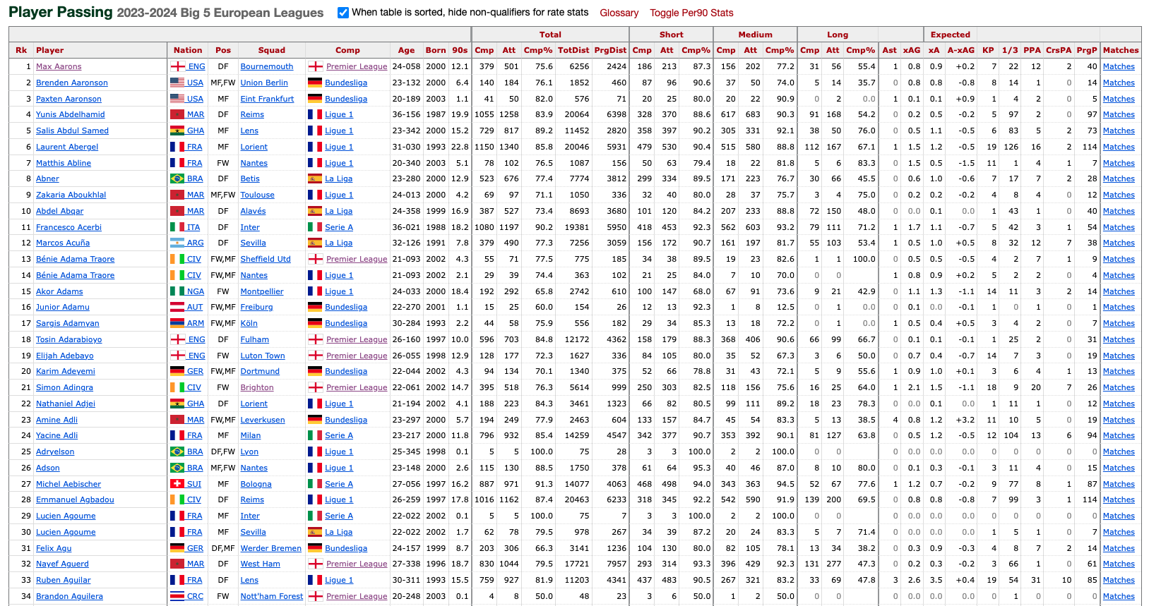
However, the catch is the types of data are split in to further sub-tables that are group by the ‘type’ of statistics, these type are:

In this post I will scrape all of these tables and combine them into 1 master table which we can save down and use for further analysis or visualisation.

Setup

Here are some of the key modules that are required in order to run this script. This Python script imports libraries for web scraping, data analysis, visualization, and machine learning. It configures the visualization environment, sets display options, and imports image processing modules.

import os
import requests
import pandas as pd
from bs4 import BeautifulSoup
import seaborn as sb
import matplotlib.pyplot as plt
import matplotlib as mpl
import warnings
import numpy as np
from math import pi
from urllib.request import urlopen
import matplotlib.patheffects as pe
from highlight_text import fig_text
from adjustText import adjust_text
from tabulate import tabulate
import matplotlib.style as style
import unicodedata
from fuzzywuzzy import fuzz
from fuzzywuzzy import process
import matplotlib.ticker as ticker
import matplotlib.patheffects as path_effects
import matplotlib.font_manager as fm
import matplotlib.colors as mcolors
from matplotlib import cm
from highlight_text import fig_text

import matplotlib.pyplot as plt
import seaborn as sns
%matplotlib inline

from sklearn import preprocessing

style.use('fivethirtyeight')

from PIL import Image
import urllib
import os
import math
from PIL import Image
import matplotlib.image as image

Data Preparation & Constructing Functions

The code below defines a function called position_grouping that takes a player’s position (x) as input. It categorizes players into different position groups based on their positions, such as goalkeepers (GK), defenders, wing-backs, defensive midfielders, central midfielders, attacking midfielders, and forwards.

The function uses conditional statements (if-elif-else) to determine the appropriate position group for a given input position. If the input matches any predefined positions for a group, it returns the corresponding group name. If the position doesn’t match any predefined groups, it returns “unidentified position.” The purpose is to classify football players into broader position categories for easier analysis or grouping.

keepers = ['GK']
defenders = ["DF",'DF,MF']
wing_backs = ['FW,DF','DF,FW']
defensive_mids = ['MF,DF']
midfielders = ['MF']
attacking_mids = ['MF,FW',"FW,MF"]
forwards = ['FW']

def position_grouping(x):
    if x in keepers:
        return "GK"
    elif x in defenders:
        return "Defender"
    elif x in wing_backs:
        return "Wing-Back"
    elif x in defensive_mids:
        return "Defensive-Midfielders"
    elif x in midfielders:
        return "Central Midfielders"
    elif x in attacking_mids:
        return "Attacking Midfielders"
    elif x in forwards:
        return "Forwards"
    else:
        return "unidentified position"

The next code block is basis upon which we will use to build our database creator function. I will use the pass metrics pages as the example -

This code starts by scraping passing statistics from a specified URL using the requests library and parsing the HTML content with BeautifulSoup.

The HTML content is then cleaned to remove comments and stored as a string.

The cleaned HTML content is read into a pandas DataFrame using pd.read_html(). The script modifies the DataFrame to handle multi-level column headers and assigns appropriate prefixes to distinguish passing metrics (Total, Short, Medium, Long).

Finally, it filters out rows where the ‘Player’ column is not populated, likely removing headers and irrelevant information, to prepare the DataFrame for further analysis.

    # Passing columns 
pass_ = 'https://fbref.com/en/comps/9/passing/Premier-League-Stats'
page =requests.get(pass_)
soup = BeautifulSoup(page.content, 'html.parser')
html_content = requests.get(pass_).text.replace('<!--', '').replace('-->', '')
pass_df = pd.read_html(html_content)
pass_df[-1].columns = pass_df[-1].columns.droplevel(0)
pass_stats = pass_df[-1]
pass_prefixes = {1: 'Total - ', 2: 'Short - ', 3: 'Medium - ', 4: 'Long - '}
pass_column_occurrences = {'Cmp': 0, 'Att': 0, 'Cmp%': 0}
pass_new_column_names = []
for col_name in pass_stats.columns:
    if col_name in pass_column_occurrences:
        pass_column_occurrences[col_name] += 1
        prefix = pass_prefixes[pass_column_occurrences[col_name]]
        pass_new_column_names.append(prefix + col_name)
    else:
        pass_new_column_names.append(col_name)
pass_stats.columns = pass_new_column_names
pass_stats = pass_stats[pass_stats['Player'] != 'Player']

This Python function create_full_stats_db() retrieves various football statistics from different URLs, cleans and processes the data, and merges them into a single DataFrame for comprehensive analysis:

1: Passing Statistics: Retrieves passing data from a URL, processes it to handle multi-level column headers, and renames columns with appropriate prefixes.

2: Shooting Statistics: Fetches shooting data, cleans it by dropping irrelevant rows, and stores it.

3: Passing Type Statistics: Gathers passing type data, cleans column headers, and stores it.

4: Goal Creation & Assists Statistics (GCA): Fetches GCA data, processes column headers, and stores it.

4: Defensive Statistics: Retrieves defensive data, renames columns, and stores it.

5: Possession Statistics: Gathers possession-related data, renames columns, and stores it.

6: Miscellaneous Statistics: Retrieves miscellaneous data, cleans it, and stores it.

7: Merging DataFrames: Merges all the data frames on common player attributes, such as name, nationality, position, squad, age, and playing time.

8: Data Cleaning: Handles missing values, converts non-numeric columns to numeric where possible, and adds a column for position grouping using the previously defined position_grouping function.

9: Returns: Returns the merged and cleaned DataFrame containing all the football statistics for further analysis.

Here is the full function below:

def create_full_stats_db():
    # Passing columns 
    pass_ = 'https://fbref.com/en/comps/9/passing/Premier-League-Stats'
    page =requests.get(pass_)
    soup = BeautifulSoup(page.content, 'html.parser')
    html_content = requests.get(pass_).text.replace('<!--', '').replace('-->', '')
    pass_df = pd.read_html(html_content)
    pass_df[-1].columns = pass_df[-1].columns.droplevel(0)
    pass_stats = pass_df[-1]
    pass_prefixes = {1: 'Total - ', 2: 'Short - ', 3: 'Medium - ', 4: 'Long - '}
    pass_column_occurrences = {'Cmp': 0, 'Att': 0, 'Cmp%': 0}
    pass_new_column_names = []
    for col_name in pass_stats.columns:
        if col_name in pass_column_occurrences:
            pass_column_occurrences[col_name] += 1
            prefix = pass_prefixes[pass_column_occurrences[col_name]]
            pass_new_column_names.append(prefix + col_name)
        else:
            pass_new_column_names.append(col_name)
    pass_stats.columns = pass_new_column_names
    pass_stats = pass_stats[pass_stats['Player'] != 'Player']

    # Shooting columns 
    shot_ = 'https://fbref.com/en/comps/9/shooting/Premier-League-Stats'
    page =requests.get(shot_)
    soup = BeautifulSoup(page.content, 'html.parser')
    html_content = requests.get(shot_).text.replace('<!--', '').replace('-->', '')
    shot_df = pd.read_html(html_content)
    shot_df[-1].columns = shot_df[-1].columns.droplevel(0) # drop top header row
    shot_stats = shot_df[-1]
    shot_stats = shot_stats[shot_stats['Player'] != 'Player']    



    # Pass Type columns 
    pass_type = 'https://fbref.com/en/comps/9/passing_types/Premier-League-Stats'
    page =requests.get(pass_type)
    soup = BeautifulSoup(page.content, 'html.parser')
    html_content = requests.get(pass_type).text.replace('<!--', '').replace('-->', '')
    pass_type_df = pd.read_html(html_content)
    pass_type_df[-1].columns = pass_type_df[-1].columns.droplevel(0) # drop top header row
    pass_type_stats = pass_type_df[-1]
    pass_type_stats = pass_type_stats[pass_type_stats['Player'] != 'Player']


    # GCA columns 
    gca_ = 'https://fbref.com/en/comps/9/gca/Premier-League-Stats'
    page =requests.get(gca_)
    soup = BeautifulSoup(page.content, 'html.parser')
    html_content = requests.get(gca_).text.replace('<!--', '').replace('-->', '')
    gca_df = pd.read_html(html_content)
    gca_df[-1].columns = gca_df[-1].columns.droplevel(0)
    gca_stats = gca_df[-1]
    gca_prefixes = {1: 'SCA - ', 2: 'GCA - '}
    gca_column_occurrences = {'PassLive': 0, 'PassDead': 0, 'TO%': 0, 'Sh': 0, 'Fld': 0, 'Def': 0}
    gca_new_column_names = []
    for col_name in gca_stats.columns:
        if col_name in gca_column_occurrences:
            gca_column_occurrences[col_name] += 1
            prefix = gca_prefixes[gca_column_occurrences[col_name]]
            gca_new_column_names.append(prefix + col_name)
        else:
            gca_new_column_names.append(col_name)
    gca_stats.columns = gca_new_column_names
    gca_stats = gca_stats[gca_stats['Player'] != 'Player']
    

    # Defense columns 
    defence_ = 'https://fbref.com/en/comps/9/defense/Premier-League-Stats'
    page =requests.get(defence_)
    soup = BeautifulSoup(page.content, 'html.parser')
    html_content = requests.get(defence_).text.replace('<!--', '').replace('-->', '')
    defence_df = pd.read_html(html_content)
    defence_df[-1].columns = defence_df[-1].columns.droplevel(0) # drop top header row
    defence_stats = defence_df[-1]
    rename_columns = {
    'Def 3rd': 'Tackles - Def 3rd',
    'Mid 3rd': 'Tackles - Mid 3rd',
    'Att 3rd': 'Tackles - Att 3rd',
    'Blocks': 'Total Blocks',
    'Sh': 'Shots Blocked',
    'Pass': 'Passes Blocked'}
    defence_stats.rename(columns = rename_columns, inplace=True)
    defence_prefixes = {1: 'Total - ', 2: 'Dribblers- '}
    defence_column_occurrences = {'Tkl': 0}
    new_column_names = []
    for col_name in defence_stats.columns:
        if col_name in defence_column_occurrences:
            defence_column_occurrences[col_name] += 1
            prefix = defence_prefixes[defence_column_occurrences[col_name]]
            new_column_names.append(prefix + col_name)
        else:
            new_column_names.append(col_name)
    defence_stats.columns = new_column_names
    defence_stats = defence_stats[defence_stats['Player'] != 'Player']


    # possession columns 
    poss_ = 'https://fbref.com/en/comps/9/possession/Premier-League-Stats'
    page =requests.get(poss_)
    soup = BeautifulSoup(page.content, 'html.parser')
    html_content = requests.get(poss_).text.replace('<!--', '').replace('-->', '')
    poss_df = pd.read_html(html_content)
    poss_df[-1].columns = poss_df[-1].columns.droplevel(0) # drop top header row
    poss_stats = poss_df[-1]
    rename_columns = {
    'TotDist': 'Carries - TotDist',
    'PrgDist': 'Carries - PrgDist',
    'PrgC': 'Carries - PrgC',
    '1/3': 'Carries - 1/3',
    'CPA': 'Carries - CPA',
    'Mis': 'Carries - Mis',
    'Dis': 'Carries - Dis',
    'Att': 'Take Ons - Attempted'  }
    poss_stats.rename(columns=rename_columns, inplace=True)
    poss_stats = poss_stats[poss_stats['Player'] != 'Player']


    # misc columns 
    misc_ = 'https://fbref.com/en/comps/9/misc/Premier-League-Stats'
    page =requests.get(misc_)
    soup = BeautifulSoup(page.content, 'html.parser')
    html_content = requests.get(misc_).text.replace('<!--', '').replace('-->', '')
    misc_df = pd.read_html(html_content)
    misc_df[-1].columns = misc_df[-1].columns.droplevel(0) # drop top header row
    misc_stats = misc_df[-1]
    misc_stats = misc_stats[misc_stats['Player'] != 'Player']

    index_df = misc_stats[['Player', 'Nation', 'Pos', 'Squad', 'Age', 'Born', '90s']]

    data_frames = [poss_stats, misc_stats, pass_stats ,defence_stats, shot_stats, gca_stats, pass_type_stats]
    for df in data_frames:
        if df is not None:  # Checking if the DataFrame exists
            df.drop(columns=['Matches', 'Rk'], inplace=True, errors='ignore')
            df.dropna(axis=0, how='any', inplace=True)

            index_df = pd.merge(index_df, df, on=['Player', 'Nation', 'Pos', 'Squad', 'Age', 'Born', '90s'], how='left')
    index_df["position_group"] = index_df.Pos.apply(lambda x: position_grouping(x))  

    index_df.fillna(0, inplace=True)

    non_numeric_cols = ['Player', 'Nation', 'Pos', 'Squad', 'Age', 'position_group']
    
    def clean_non_convertible_values(value):
        try:
            return pd.to_numeric(value)
        except (ValueError, TypeError):
            return np.nan

    # Iterate through each column, converting non-numeric columns to numeric
    for col in index_df.columns:
        if col not in non_numeric_cols:
            index_df[col] = index_df[col].apply(clean_non_convertible_values)

    
    return index_df

Now that we have our function, we can now store all of the relevant pages as variables and pass them into out function arguments of the function. The variables can be stored as follows:

fbref_passing = 'https://fbref.com/en/comps/Big5/passing/players/Big-5-European-Leagues-Stats'
fbref_shooting = 'https://fbref.com/en/comps/Big5/shooting/players/Big-5-European-Leagues-Stats'
fbref_pass_type = 'https://fbref.com/en/comps/Big5/passing_types/players/Big-5-European-Leagues-Stats'
fbref_defence = 'https://fbref.com/en/comps/Big5/defense/players/Big-5-European-Leagues-Stats'
fbref_gca = 'https://fbref.com/en/comps/Big5/gca/players/Big-5-European-Leagues-Stats'
fbref_poss = 'https://fbref.com/en/comps/Big5/possession/players/Big-5-European-Leagues-Stats'
fbref_misc = 'https://fbref.com/en/comps/Big5/misc/players/Big-5-European-Leagues-Stats'

stats = create_full_stats_db(fbref_passing,fbref_shooting,fbref_pass_type,fbref_defence,fbref_gca,fbref_poss,fbref_misc)

We have now created a relatively simple function that is able to retrieve all key player data from FBREF in under 11 seconds, meaning that this data can easily be refreshed with minimal effort.

Comparing Player Passing Stats

The code effectively pre-processes and selects data relevant for further analysis, focusing on key passing and assist statistics per 90 minutes, and identifies the top players based on their expected goal contributions. Here are the following operations:

Selection of Columns: Selects specific columns (‘Player’, ‘position_group’, ‘KP’, ‘PPA’, ‘PrgDist’, ‘Total - Cmp%’, ’90s’, ‘A-xAG’, ‘xA’, ‘xAG’) from the DataFrame stats and assigns the resulting DataFrame to Player_stats.
Filtering Rows: Filters out rows where the ‘Player’ column is populated with ‘Player’, presumably removing header rows.
Drop Missing Values: Drops rows where the ‘KP’ column has missing values (NaN).
Calculations:
- Calculates ‘Key Passes per 90’ by dividing ‘KP’ (Key Passes) by ’90s’ (Minutes played divided by 90).
- Calculates ‘PPA_p90’ (Passes into Penalty Area per 90) by dividing ‘PPA’ (Passes into Penalty Area) by ’90s’.
- Calculates ‘Expected Assists per 90’ by dividing ‘xA’ (Expected Assists) by ’90s’.
Filtering by Playing Time: Filters out players who have played less than 4.5 full matches (90 minutes each).
Top Players: Selects the top 10 players with the highest ‘xAG’ (Expected Goals Assisted) values and stores their names in the list ‘players’.

Player_stats = stats[['Player','position_group', 'KP','PPA', 'PrgDist', 'Total - Cmp%', '90s','A-xAG','xA', 'xAG']]
Player_stats = Player_stats[Player_stats['Player'] != 'Player']
Player_stats.dropna(subset=['KP'], inplace=True)
Player_stats['Key Passes per 90'] = Player_stats['KP']/Player_stats['90s']
Player_stats['PPA_p90'] = Player_stats['PPA']/Player_stats['90s']
Player_stats['Expected Assists per 90'] = Player_stats['xA']/Player_stats['90s']
Player_stats = Player_stats[Player_stats['90s'] >= 4.5]
top_7 = Player_stats.nlargest(10, 'xAG')
players = top_7['Player'].tolist()

These variables are to be used in conjunction with a Player_stats dataframe:

x_var: This variable represents the x-axis variable for the plot. It is set to Key Passes per 90.
y_var: This variable represents the y-axis variable for the plot. It is set to Expected Assists per 90.
Title: This variable holds a string representing the title for the visualization or analysis. It’s formatted with line breaks and angle brackets for emphasis and readability.

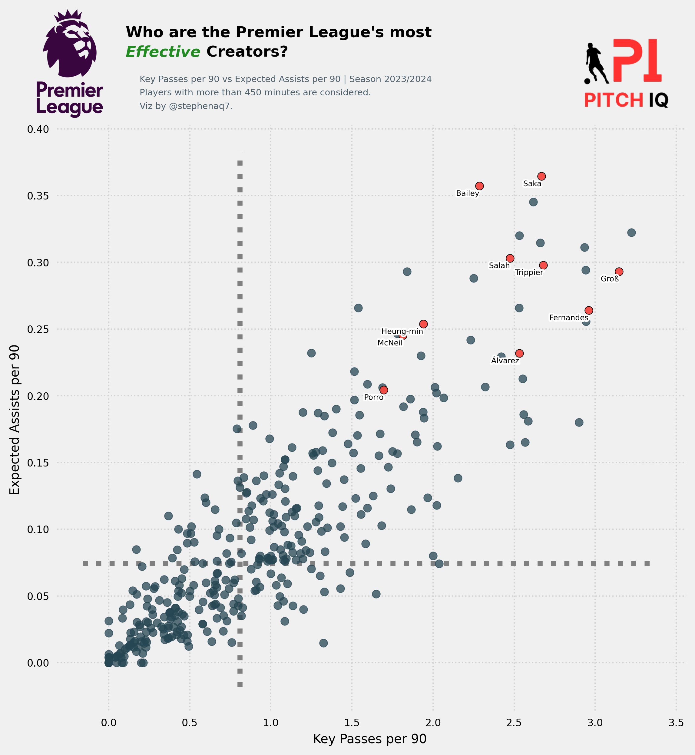
x_var = 'Key Passes per 90'
y_var = 'Expected Assists per 90'
Title = "Who are the Premier League's most\n<Effective> Creators?"

This next function create_scatter_plot() generates a scatter plot comparing two variables (x_var and y_var) from the Player_stats dataframe . Here’s a breakdown of what it does:

Splitting Data: It splits the Player_stats DataFrame into two DataFrames:
- df_main: Contains players who are not in the list players.
- df_highlight: Contains players who are in the list players.
Plotting the Chart:
- Sets up the figure and axis for the plot.
- Plots the main data points (players not in players) as scatter points in blue (#264653).
- Plots the highlighted data points (players in players) as scatter points in red (#F64740) with black edges.
- Adds median lines for both x and y variables in gray.
- Adds a light gray grid.
Annotations:
- Annotates each highlighted player’s data point with their last name (splitting on space) at a specific offset.
- Adds a stroke effect to the text for better visibility.
Axis Labels and Tick Sizes: Sets axis labels and tick sizes.
League Icon: Adds the Premier League icon as an image in the top left corner.
Title and Description: Adds a title and description to the plot.
PitchIQ Logo: Adds a logo at the bottom right corner of the plot.

Overall, this function creates a visually appealing scatter plot comparing two variables for a selected set of football players, with special emphasis on certain highlighted players

Here is step by step guide of what each code block is trying to perform:

1: Splitting Data:

df_main = Player_stats[~Player_stats["Player"].isin(players)].reset_index(drop = True)
df_highlight = Player_stats[Player_stats["Player"].isin(players)].reset_index(drop = True)

Splits the Player_stats DataFrame into two DataFrames:
- df_main: Contains players who are not in the list players.
- df_highlight: Contains players who are in the list players.

2: Plotting the Chart:

fig = plt.figure(figsize = (8,8), dpi = 300)
ax = plt.subplot()

Sets up the figure and axis for the plot.

3: Styling the Plot:

ax.spines["top"].set_visible(False)
ax.spines["right"].set_visible(False)

Removes the top and right spines of the plot.

4: Scatter Plots:

ax.scatter(
    df_main[x_var],
    df_main[y_var],  
    s = 40, 
    alpha = 0.75, 
    color = "#264653",
    zorder = 3
)

Plots the main data points (players not in players) as scatter points in blue (#264653).

ax.scatter(
    df_highlight[x_var], 
    df_highlight[y_var], 
    s = 40, 
    alpha = 0.95, 
    color = "#F64740",
    zorder = 3,
    ec = "#000000",
)

Plots the highlighted data points (players in players) as scatter points in red (#F64740) with black edges.

5: Median Lines:

ax.plot(
    [Player_stats[x_var].median(), Player_stats[x_var].median()],
    [ax.get_ylim()[0], ax.get_ylim()[1]], 
    ls = ":",
    color = "gray",
    zorder = 2
)

Adds a median line for the x-variable in gray.

ax.plot(
    [ax.get_xlim()[0], ax.get_xlim()[1]],
    [Player_stats[y_var].median(), Player_stats[y_var].median()], 
    ls = ":",
    color = "gray",
    zorder = 2
)

Adds a median line for the y-variable in gray.

6: Grid:

ax.grid(True, ls = ":", color = "lightgray")

Adds a light gray grid.

7: Annotations:

Iterates through each highlighted player’s data point, annotating their last name next to the point.
Applies a stroke effect to the text for better visibility.

8: Axis Labels and Tick Sizes:

ax.set_xlabel(x_var,fontsize=10)
ax.set_ylabel(y_var,fontsize=10)
ax.tick_params(axis='both', which='major', labelsize=8)

Sets axis labels and tick sizes.

9: League Icon:

league_icon = Image.open("/Users/stephenahiabah/Desktop/GitHub/Webs-scarping-for-Fooball-Data-/Images/premier-league-2-logo.png")
league_ax = fig.add_axes([0.002, 0.89, 0.20, 0.15], zorder=1)
league_ax.imshow(league_icon)
league_ax.axis("off")

Adds the Premier League icon as an image in the top left corner.

10: Title and Description:

fig_text(
    x = 0.60, y = 0.97, 
    s = Title,
    highlight_textprops=[{"color":"#228B22", "style":"italic"}],
    va = "bottom", ha = "right",
    fontsize = 12, color = "black", font = "Karla", weight = "bold"
)

fig_text(
    x = 0.60, y = .90, 
    s = f"{x_var} vs {y_var} | Season 2023/2024\nPlayers with more than 450 minutes are considered.\nViz by @stephenaq7.",
    va = "bottom", ha = "right",
    fontsize = 7, color = "#4E616C", font = "Karla"
)

Adds a title and description to the plot.

11: Stats by PitchIQ Logo:

ax3 = fig.add_axes([0.80, 0.08, 0.13, 1.75])
ax3.axis('off')
img = image.imread('/Users/stephenahiabah/Desktop/GitHub/Webs-scarping-for-Fooball-Data-/outputs/piqmain.png')
ax3.imshow(img)

Adds a logo at the bottom right corner of the plot.

Here is the code in full below;

def create_scatter_plot(players,Player_stats,x_var,y_var,Title):    
    df_main = Player_stats[~Player_stats["Player"].isin(players)].reset_index(drop = True)
    df_highlight = Player_stats[Player_stats["Player"].isin(players)].reset_index(drop = True)

    # %%

    # -- Plot the chart

    fig = plt.figure(figsize = (8,8), dpi = 300)
    ax = plt.subplot()

    ax.spines["top"].set_visible(False)
    ax.spines["right"].set_visible(False)

    ax.scatter(
        df_main[x_var],
        df_main[y_var],  
        s = 40, 
        alpha = 0.75, 
        color = "#264653",
        zorder = 3
    )

    ax.scatter(
        df_highlight[x_var], 
        df_highlight[y_var], 
        s = 40, 
        alpha = 0.95, 
        color = "#F64740",
        zorder = 3,
        ec = "#000000",
    )

    ax.plot(
        [Player_stats[x_var].median(), Player_stats[x_var].median()],
        [ax.get_ylim()[0], ax.get_ylim()[1]], 
        ls = ":",
        color = "gray",
        zorder = 2
    )

    ax.plot(
        [ax.get_xlim()[0], ax.get_xlim()[1]],
        [Player_stats[y_var].median(), Player_stats[y_var].median()], 
        ls = ":",
        color = "gray",
        zorder = 2
    )

    ax.grid(True, ls = ":", color = "lightgray")

    for index, name in enumerate(df_highlight["Player"]):
        X = df_highlight[x_var].iloc[index]
        Y = df_highlight[y_var].iloc[index]
        if name in [" Joelinton", " Richarlison", "Alexandre Lacazette"]:
            y_pos = 9
        else:
            y_pos = -9
        if name in ["Scott McTominay"]:
            x_pos = 20
        else:
            x_pos = 0
        text_ = ax.annotate(
            xy = (X, Y),
            text = name.split(" ")[1],
            ha = "right",
            va = "bottom",
            xytext = (x_pos, y_pos),
            textcoords = "offset points",
            fontsize=6, 
        )

        text_.set_path_effects(
                    [path_effects.Stroke(linewidth=2.5, foreground="white"), 
                    path_effects.Normal()]
                )


    ax.set_xlabel(x_var,fontsize=10)
    ax.set_ylabel(y_var,fontsize=10)

    league_icon = Image.open("/Users/stephenahiabah/Desktop/GitHub/Webs-scarping-for-Fooball-Data-/Images/premier-league-2-logo.png")
    league_ax = fig.add_axes([0.002, 0.89, 0.20, 0.15], zorder=1)
    league_ax.imshow(league_icon)
    league_ax.axis("off")

    ax.tick_params(axis='both', which='major', labelsize=8)

    fig_text(
        x = 0.60, y = 0.97, 
        s = Title,
        highlight_textprops=[{"color":"#228B22", "style":"italic"}],
        va = "bottom", ha = "right",
        fontsize = 12, color = "black", font = "Karla", weight = "bold"
    )

    fig_text(
        x = 0.60, y = .90, 
        s = f"{x_var} vs {y_var} | Season 2023/2024\nPlayers with more than 450 minutes are considered.\nViz by @stephenaq7.",
        va = "bottom", ha = "right",
        fontsize = 7, color = "#4E616C", font = "Karla"
    )

    ### Add Stats by Steve logo
    ax3 = fig.add_axes([0.80, 0.08, 0.13, 1.75])
    ax3.axis('off')
    img = image.imread('/Users/stephenahiabah/Desktop/GitHub/Webs-scarping-for-Fooball-Data-/outputs/piqmain.png')
    ax3.imshow(img)

Comparing Player Shooting Stats

We’ll now perfrom the same type of aggregations with player shooting statistics to create a similar scatter plot.

Player_stats = stats[['Player','position_group', 'SoT/90', 'xG','90s',
 'npxG',
 'npxG/Sh',
 'G-xG',
 'np:G-xG']]
Player_stats['Shots on Target per 90'] = Player_stats['SoT/90']
Player_stats['Non-Penalty xG per 90'] = Player_stats['npxG']/Player_stats['90s']
Player_stats = Player_stats[Player_stats['90s'] >= 4.5]
top_7 = Player_stats.nlargest(10, 'xG')
players = top_7['Player'].tolist()

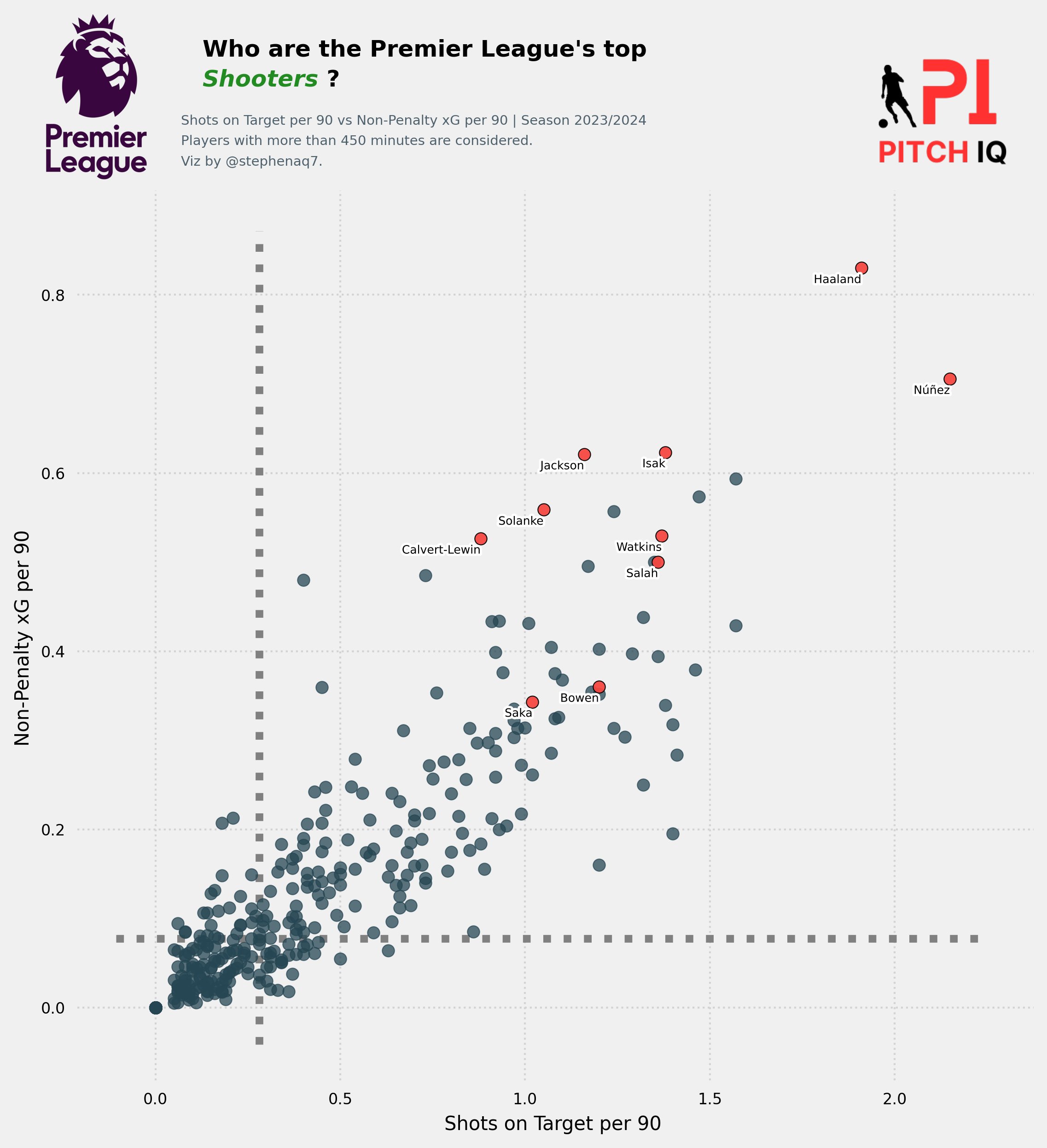
x_var = 'Shots on Target per 90'
y_var = 'Non-Penalty xG per 90'
Title = "Who are the Premier League's top\n<Shooters> ?"

The resulting plot should look like the following:

create_scatter_plot(players,Player_stats,x_var,y_var,Title)

Creating Purpose Built Metrics Scores with sk.learn

In all my previous posts I have large focused on creting detailed visualisations and webscaping data. As a statitician by trade, I’ll now be foucssing on more data science/ statistics applications when using data from FBREF. I have recently been building a playing rating model/ similarity model. This next part of the tutorial will focus on how I building a rudimentary version of my player scoring model.

Let me breakdown the reasons why its powerful to create metrics derived from the raw data scraped from FBREF:

Creating your own scores using data from FBREF can be immensely useful for several reasons. Firstly, FBREF provides a vast array of detailed statistics on player performance, covering various aspects of the game such as passing accuracy, defensive actions, creativity, and shooting efficiency.
By aggregating and analyzing these statistics, you can develop customized scoring metrics tailored to specific performance attributes or player roles, allowing for more nuanced and insightful evaluations. Additionally, creating your own scores enables you to focus on metrics that are most relevant to your analysis or decision-making process, rather than relying solely on standardized metrics provided by external sources.
This approach can offer a deeper understanding of player contributions, strengths, and weaknesses, facilitating more informed decisions in areas such as player recruitment, team selection, tactical adjustments, and performance evaluation. Moreover, developing custom scoring systems allows for flexibility and adaptation to evolving strategies, player roles, and performance trends, enhancing the relevance and applicability of the analysis in various contexts within football management and analytics.

Selecting Features:

The provided code below defines two lists: non_numeric_cols and key_stats.

non_numeric_cols: This list contains the names of columns in a dataset that are considered non-numeric or categorical. These columns likely contain textual or categorical information about the players, such as their names, nationality, position, squad, age, and position group. These columns are typically not used for numerical calculations or statistical analysis but are often important for identifying and categorizing players.
key_stats: This list contains the names of columns in a dataset that represent key performance metrics or statistics related to football player performance. These metrics include statistics such as playing time (90s), passing accuracy (Total - Cmp%), key passes (KP), tackles (Tkl), blocks (Total Blocks), expected goals (xG), shots on target (SoT), and others. These metrics are typically numerical and are essential for analyzing and evaluating player performance on the field. They provide insights into various aspects of a player’s contributions to the team and are commonly used in football analytics and performance evaluation.

non_numeric_cols = ['Player', 'Nation', 'Pos', 'Squad', 'Age', 'position_group']
key_stats = ['90s','Total - Cmp%','KP', 'TB','Sw','PPA', 'PrgP','Tkl%','Total Blocks', 'Tkl+Int','Clr', 'Carries - PrgDist','SCA90','GCA90','CrsPA','xA', 'Rec','PrgR','xG', 'Sh','SoT']

In this example we’ll be looking at defenders seeing as we’ve already covered strikers and creative midfielders in previous examples

The provided code below performs several operations on a DataFrame named stats:

stats.dropna(axis=0, how='any', inplace=True): This line drops rows with any missing values (NaN) across all columns in the DataFrame, ensuring that the DataFrame contains only complete data.
defender_stats = stats[stats['position_group'] == 'Defender']: This line filters the DataFrame to include only rows where the value in the ‘position_group’ column is equal to ‘Defender’, creating a new DataFrame named defender_stats.
defender_stats = defender_stats[non_numeric_cols + key_stats]: This line selects specific columns from the defender_stats DataFrame, including both non-numeric columns (listed in non_numeric_cols) and key statistics columns (listed in key_stats). It creates a new DataFrame containing only these selected columns.
defender_stats = defender_stats[defender_stats['90s'] > 5]: This line further filters the defender_stats DataFrame to include only rows where the value in the ’90s’ column (representing playing time) is greater than 5, indicating that the player has played more than 5 complete matches. This filter likely aims to focus the analysis on defenders who have significant playing time on the field.

Dataframe Manipulation:

stats.dropna(axis=0, how='any', inplace=True)
defender_stats = stats[stats['position_group'] == 'Defender']
defender_stats = defender_stats[non_numeric_cols + key_stats]
defender_stats = defender_stats[defender_stats['90s'] > 5]

This next code block comprises of a function that essentially performs a per-90-minute normalization for numeric columns in the DataFrame, excluding certain columns and handling division by zero cases.

Here’s a breakdown of the code per_90fi:

1: Fill NaN Values:

Replaces all NaN values in the DataFrame with 0.

   dataframe = dataframe.fillna(0)

2: Identify Numeric Columns:

Finds all columns in the DataFrame that contain numeric data.

   numeric_columns = [col for col in dataframe.columns if np.issubdtype(dataframe[col].dtype, np.number)]

3: Exclude Columns:

Specifies columns to exclude from normalization, such as player names, nationality, position, squad, age, birth year, position group, and the column ’90s’ (presumably representing minutes played).

   exclude_columns = ['Player', 'Nation', 'Pos', 'Squad', 'Age', 'Born', 'position_group','90s']

4: Identify Columns to Divide:

Identifies numeric columns to divide by the ’90s’ column.
Excludes columns containing ‘90’ or ‘%’ in their names.

   columns_to_divide = [col for col in numeric_columns if col not in exclude_columns 
                         and '90' not in col and '%' not in col and '90s' not in col]

5: Create a Mask:

Creates a boolean mask to avoid division by zero or blank values for the ’90s’ column.

   mask = (dataframe['90s'] != 0)

6: Normalize Data:

Divides each identified column by the ’90s’ column, handling division by zero or blank values.

   for col in columns_to_divide:
       dataframe.loc[mask, col] /= dataframe.loc[mask, '90s']

7: Return DataFrame:

Returns the modified DataFrame after normalization.

Here is the full code below:

def per_90fi(dataframe):
    # Replace empty strings ('') with NaN
    # dataframe = dataframe.replace('', np.nan)
    
    # Fill NaN values with 0
    dataframe = dataframe.fillna(0)
    
    # Convert numeric columns to numeric type
    numeric_columns = [col for col in dataframe.columns if np.issubdtype(dataframe[col].dtype, np.number)]
    numeric_columns = [value for value in numeric_columns if value != "90s"]
    
    # Exclude specified columns from the normalization
    exclude_columns = ['Player', 'Nation', 'Pos', 'Squad', 'Age', 'Born', 'position_group','90s']
    
    # Identify numeric columns to divide by '90s' and exclude columns with '%' and '90' in their names
    columns_to_divide = [col for col in numeric_columns if col not in exclude_columns 
                         and '90' not in col and '%' not in col and '90s' not in col]
    
    # Create a mask to avoid division by zero or blank values
    mask = (dataframe['90s'] != 0) 
    
    # Divide each identified column by the '90s' column, handling division by zero or blank values

    for col in columns_to_divide:
        dataframe.loc[mask, col] /= dataframe.loc[mask, '90s']

    return dataframe

# Assuming 'your_dataframe' contains your dataset
# Call the function to perform the normalization
defender_stats = per_90fi(defender_stats)

The code begins by importing necessary libraries and defining lists for different types of metrics. It then utilizes MinMaxScaler to normalize the core statistics, calculates mean scores for passing, defending, creation, and shooting metrics for each player, adds offsets to ensure uniqueness, and clips the scores to a range of 0 to 10. After adjusting player ratings to a desired range, it applies these functions to the data, generating comprehensive scoring metrics for each player. Finally, it merges the original dataset with the computed scores, providing a consolidated dataset for further analysis and comparison.

Here’s a step-by-step explanation of the provided code:

1: Import Libraries:

Import necessary libraries including Pandas for data manipulation and MinMaxScaler from sklearn.preprocessing for feature scaling.

   import pandas as pd
   from sklearn.preprocessing import MinMaxScaler

2: Define Metrics Lists:

Define lists for different types of metrics including core statistics, passing metrics, defending metrics, creation metrics, and shooting metrics.

   core_stats = ['90s', 'Total - Cmp%', 'KP', 'TB', 'Sw', 'PPA', 'PrgP', 'Tkl%', 'Total Blocks', 'Tkl+Int', 'Clr', 'Carries - PrgDist', 'SCA90', 'GCA90', 'CrsPA', 'xA', 'Rec', 'PrgR', 'xG', 'Sh', 'SoT']
   passing_metrics = ['Total - Cmp%', 'KP', 'TB', 'Sw', 'PPA', 'PrgP']
   defending_metrics = ['Tkl%', 'Total Blocks', 'Tkl+Int', 'Clr']
   creation_metrics = ['Carries - PrgDist', 'SCA90', 'GCA90', 'CrsPA', 'xA', 'Rec', 'PrgR']
   shooting_metrics = ['xG', 'Sh', 'SoT']

3: Create a MinMaxScaler Instance:

Instantiate a MinMaxScaler object to scale the data.

   scaler = MinMaxScaler()

4: Normalize the Metrics:

Make a copy of the DataFrame.
Normalize the values of core statistics using Min-Max scaling.

   stats_normalized = df.copy()
   stats_normalized[core_stats] = scaler.fit_transform(stats_normalized[core_stats])

5: Calculate Scores for Each Metric Grouping:

Calculate the mean of passing, defending, creation, and shooting metrics for each player.
Scale the mean scores to a range of 0-10.

   stats_normalized['Passing_Score'] = stats_normalized[passing_metrics].mean(axis=1) * 10
   stats_normalized['Defending_Score'] = stats_normalized[defending_metrics].mean(axis=1) * 10
   stats_normalized['Creation_Score'] = stats_normalized[creation_metrics].mean(axis=1) * 10
   stats_normalized['Shooting_Score'] = stats_normalized[shooting_metrics].mean(axis=1) * 10

6: Add an Offset and Clip Scores:

Add a small offset to ensure unique scores.
Clip scores to ensure they are within the 0-10 range.

   stats_normalized['Passing_Score'] += stats_normalized.index * 0.001
   stats_normalized['Defending_Score'] += stats_normalized.index * 0.001
   stats_normalized['Creation_Score'] += stats_normalized.index * 0.001
   stats_normalized['Shooting_Score'] += stats_normalized.index * 0.001
   stats_normalized[['Passing_Score', 'Defending_Score', 'Creation_Score', 'Shooting_Score']] = stats_normalized[['Passing_Score', 'Defending_Score', 'Creation_Score', 'Shooting_Score']].clip(lower=0, upper=10)

7: Adjust Player Rating Range:

Extract the ‘total player rating’ columns.
Normalize the ratings to be within the desired range (5 to 9.5) for each column.

   for col in player_ratings.columns:
       normalized_ratings = min_rating + (max_rating - min_rating) * ((player_ratings[col] - player_ratings[col].min()) / (player_ratings[col].max() - player_ratings[col].min()))
       dataframe[col] = normalized_ratings

8: Apply the Functions to the Data:

Apply the create_metrics_scores function to generate scores for each player based on different metric groupings.
Apply the adjust_player_rating_range function to adjust the player rating range.

   pitch_iq_scoring = create_metrics_scores(defender_stats)
   pitch_iq_scoring = adjust_player_rating_range(pitch_iq_scoring)

9: Merge DataFrames:

Merge the original defender_stats DataFrame with the newly generated scores.

   defender_stats = pd.merge(defender_stats, pitch_iq_scoring, on='Player', how='left')

This code preprocesses and transforms the data to generate scores for each player based on different metric groupings and adjusts the player rating range accordingly.

Statistical Modelling

import pandas as pd
from sklearn.preprocessing import MinMaxScaler

def create_metrics_scores(df):
    # Define the key_stats grouped by the metrics
    core_stats = ['90s','Total - Cmp%','KP', 'TB','Sw','PPA', 'PrgP','Tkl%','Total Blocks', 'Tkl+Int','Clr', 'Carries - PrgDist','SCA90','GCA90','CrsPA','xA', 'Rec','PrgR','xG', 'Sh','SoT']
    passing_metrics = ['Total - Cmp%', 'KP', 'TB', 'Sw', 'PPA', 'PrgP']
    defending_metrics = ['Tkl%', 'Total Blocks', 'Tkl+Int', 'Clr']
    creation_metrics = ['Carries - PrgDist', 'SCA90', 'GCA90', 'CrsPA', 'xA', 'Rec', 'PrgR']
    shooting_metrics = ['xG', 'Sh', 'SoT']

    # Create a MinMaxScaler instance
    scaler = MinMaxScaler()

    # Normalize the metrics
    stats_normalized = df.copy()  # Create a copy of the DataFrame
    stats_normalized[core_stats] = scaler.fit_transform(stats_normalized[core_stats])

    # Calculate scores for each metric grouping and scale to 0-10
    stats_normalized['Passing_Score'] = stats_normalized[passing_metrics].mean(axis=1) * 10
    stats_normalized['Defending_Score'] = stats_normalized[defending_metrics].mean(axis=1) * 10
    stats_normalized['Creation_Score'] = stats_normalized[creation_metrics].mean(axis=1) * 10
    stats_normalized['Shooting_Score'] = stats_normalized[shooting_metrics].mean(axis=1) * 10

    # Add a small offset to ensure unique scores
    stats_normalized['Passing_Score'] += stats_normalized.index * 0.001
    stats_normalized['Defending_Score'] += stats_normalized.index * 0.001
    stats_normalized['Creation_Score'] += stats_normalized.index * 0.001
    stats_normalized['Shooting_Score'] += stats_normalized.index * 0.001

    # Clip scores to ensure they are within the 0-10 range
    stats_normalized[['Passing_Score', 'Defending_Score', 'Creation_Score', 'Shooting_Score']] = stats_normalized[['Passing_Score', 'Defending_Score', 'Creation_Score', 'Shooting_Score']].clip(lower=0, upper=10)
    return stats_normalized

def adjust_player_rating_range(dataframe):
    # Get the 'total player rating' column
    player_ratings = dataframe[['Passing_Score', 'Defending_Score', 'Creation_Score', 'Shooting_Score']]
    
    # Define the desired range for the ratings
    min_rating = 4.5
    max_rating = 9.5
    
    # Normalize the ratings to be within the desired range (5 to 9.5) for each column
    for col in player_ratings.columns:
        normalized_ratings = min_rating + (max_rating - min_rating) * ((player_ratings[col] - player_ratings[col].min()) / (player_ratings[col].max() - player_ratings[col].min()))
        dataframe[col] = normalized_ratings
    
    return dataframe


pitch_iq_scoring = create_metrics_scores(defender_stats)
pitch_iq_scoring = adjust_player_rating_range(pitch_iq_scoring)
pitch_iq_scoring = pitch_iq_scoring[['Player','Passing_Score', 'Defending_Score', 'Creation_Score', 'Shooting_Score']]
defender_stats = pd.merge(defender_stats, pitch_iq_scoring, on='Player', how='left')

The provided code extracts specific player statistics related to passing, defending, creation, and shooting scores from the ‘defender_stats’ DataFrame, sorting them based on defending scores in descending order.

Player_stats = defender_stats[['Player',
 'Nation',
 'Pos',
 'Squad',
 'Age',
'Passing_Score',
 'Defending_Score',
 'Creation_Score',
 'Shooting_Score']].sort_values(by='Defending_Score', ascending=False)

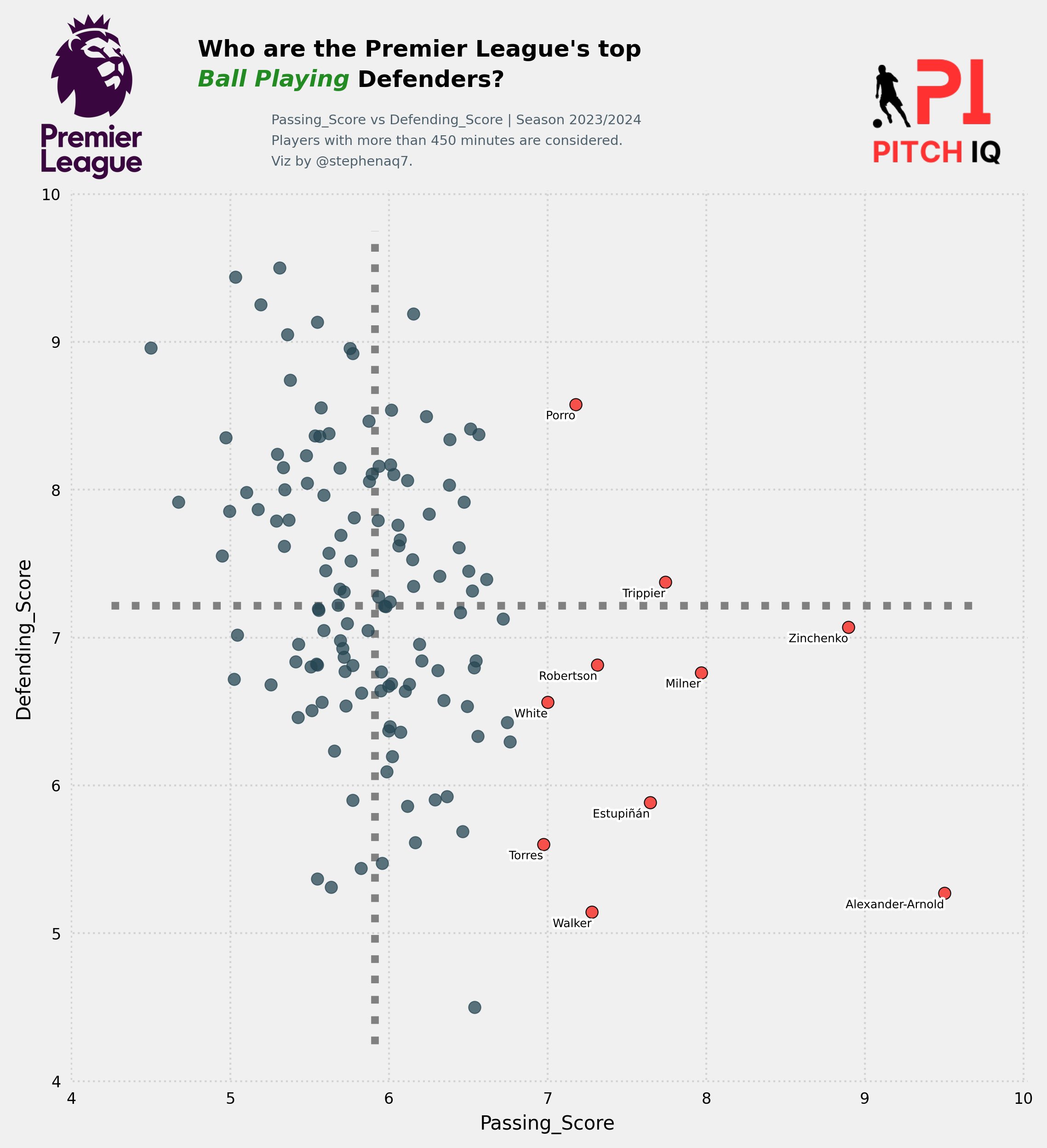
Then, we select the top 10 players with the highest passing scores and extracts their names into a list. Following this, it defines the variables ‘x_var’ and ‘y_var’ to represent passing and defending scores, respectively. Finally, it sets the title for the scatter plot visualization to inquire about the top ball-playing defenders in the Premier League, emphasizing the significance of their passing abilities.

Data Visualisation

top_7 = Player_stats.nlargest(10, 'Passing_Score')
players = top_7['Player'].tolist()
x_var = 'Passing_Score'	
y_var = 'Defending_Score'
Title = "Who are the Premier League's top\n<Ball Playing> Defenders?"

The code create_scatter_plot(players, Player_stats, x_var, y_var, Title) likely calls a function named create_scatter_plot, passing the variables players, Player_stats, x_var, y_var, and Title as arguments. This function is probably designed to generate a scatter plot visualization based on the provided data and specifications. The players variable likely contains a list of player names, Player_stats contains statistical data about these players, and x_var and y_var represent the variables to be plotted on the x and y axes, respectively. The Title variable specifies the title of the scatter plot. The function is expected to utilize these inputs to create and display the scatter plot visualization.

create_scatter_plot(players,Player_stats,x_var,y_var,Title)

The resulting plot we get looks like this:

Conclusion

In conclusion, this post serves as a valuable addition to a series of tutorials aimed at empowering users to craft dynamic and replicable functions for generating insightful data visualizations,and breif introduction into using python libraries such as sk.learn to start getting to grips with simple statistical manipulations.

Thanks for reading

Steve

PITCH IQ v3.1.2

FBREF Data Scraping - 2024 Update

Introduction

Background

Setup

Data Preparation & Constructing Functions

Comparing Player Passing Stats

Comparing Player Shooting Stats

Creating Purpose Built Metrics Scores with sk.learn

Selecting Features:

Dataframe Manipulation:

Statistical Modelling

Data Visualisation

Conclusion

Table of Contents

K-Means Player Cluster Analysis

Steve Ahiabah-Quarshie

Comments

FBREF Data Scraping - 2024 Update

Introduction

Background

Setup

Data Preparation & Constructing Functions

Comparing Player Passing Stats

Comparing Player Shooting Stats

Creating Purpose Built Metrics Scores with sk.learn

Selecting Features:

Dataframe Manipulation:

Statistical Modelling

Data Visualisation

Conclusion

Table of Contents

K-Means Player Cluster Analysis

Don't go yet!

Player Similarity Models

K-Means Player Cluster Analysis

Share

Steve Ahiabah-Quarshie

Comments