38 min to read
FBREF Data Scraping Walk Through pt3
Data analysis and visualization using scraped FBREF data
In part two of the data scraping walk through, we successfully achieved the following items;
-
Create a set of working functions to aggregate data from FBREF.
-
Perform a series of data munging tasks to get easy to to use datasets ready for analysis.
-
Create a series of Data Visualisations from these cleaned datasets.
-
Assess the meaningful metrics we need to start making some predictions on player suitability to positions.
I also added a new action to the objective of this task to:
- Build a method to programmatically access player & team level data with minimal input
In my period of research, I found sifting through the data extremely difficult. With FBREF, the webpage has been built with the User Experience of the viewers of the website in mind. I found 2 major issues when trying to build a way to easily access the data available of on the site.
- There isn’t an obvious logic to constructing the URLs of players and teams
For Example: URLs for teams in the same league look like this:
https://fbref.com/en/squads/8602292d/Aston-Villa-Stats
https://fbref.com/en/squads/47c64c55/Crystal-Palace-Stats
https://fbref.com/en/squads/b2b47a98/Newcastle-United-Stats
So, it’s not possible to just change the team name in order to get to the corect page. We need to get the correct 8 character length code in the URL (i.e: 8602292d for the Aston Villa Stats), before the team name, otherwise the URL will be invalid, in addition, these codes are unique to every page, this is also the case for player URLs, which drums up some more difficulty.
- There are drop-down menus, filters, view-toggles and various sub pages within other sub-pages that are required to access more granular data, for both Players & Teams. Each of these pages has their own unique URL.
For example, the hyperlinks at the bottom of screen grabs, show the sub-pages where all the more granular data exists:
Player Stats;
Team Stats;
There is rough pattern with these URLs, so it’s possible to write some functions to programmatically search through a database of URLs to acquire player level data in an efficient way. By using the webscraper, we can collect the URL links of sub-pages from the parent pages.
Using this basis, we can build a database of both Team and Player URLs, given the correct parent-page is accessed. Once we have the player & team URLs, we can add features like; Name, Age, Position, and playing-time. These fields will help us query the database to easily get a hold of the information we need, without having to open a webpage and copy the links every time. At the end of this exercise, key outputs we are trying to assemble are effectively 2 databases/tables. One with players and the other with teams complete with basic information and their relevant hyper-link in FBREF. This can be saved down and used whenever we want to quickly generate visualisations etc.
Setup
Let’s import all our necessary packages for web-scraping, data cleaning and analysis.
import requests
import unicodedata
import pandas as pd
from bs4 import BeautifulSoup
import seaborn as sb
import matplotlib.pyplot as plt
import matplotlib as mpl
import matplotlib.patheffects as pe
import warnings
import numpy as np
from math import pi
import os
from math import pi
from urllib.request import urlopen
from highlight_text import fig_text
from adjustText import adjust_text
from soccerplots.radar_chart import Radar
from fuzzywuzzy import fuzz
from fuzzywuzzy import process
Extra Packages to install
Before we start, there are few installations we need to do to ensure our functions work as seemlessly as possible. The links to these packages can be found below.
-
URLLIB 3 is a dependency we need in order to help us efficiently collect the URLs from the FBREF parent pages
pip install urllib3 -
Fuzzywuzzy, yes it’s actually called that. This is a handy packages that will help us match player names, if incase the player name has a foriegn (non-english) character in there e.g; Martin Ødegaard → Martin Odegaard
pip install fuzzywuzzy -
Unicodedata2 package will convert non ascii characters in player & teams names to ascii characters so when we perform our searches in the player database we need not worry about special or accented characters.
pip install unicodedata2
Building a Team & Player Database
Let’s start off with getting the team URLs. We can get the URLs of every team in a given league, from the league stats page in FBREF.
I have written a function that only requires the the URL of a league stats page to construct a dataframe of just team names and their respective URLs. So using the EPL stats page as an example, lets have a look at the output.
Getting Team URLs
def get_team_urls(x):
    url = x
    data  = requests.get(url).text
    soup = BeautifulSoup(data)
    player_urls = []
    links = BeautifulSoup(data).select('th a')
    urls = [link['href'] for link in links]
    urls = list(set(urls))
    full_urls = []
    for y in urls:
        full_url = "https://fbref.com"+y
        full_urls.append(full_url)
    team_names = []
    for team in urls:
        team_name_slice = team[20:-6]
        team_names.append(team_name_slice)
    list_of_tuples = list(zip(team_names, full_urls))
    Team_url_database = pd.DataFrame(list_of_tuples, columns = ['team_names', 'urls'])
    return Team_url_database
team_urls = get_team_urls("https://fbref.com/en/comps/9/Premier-League-Stats")
full_urls = list(team_urls.urls.unique())
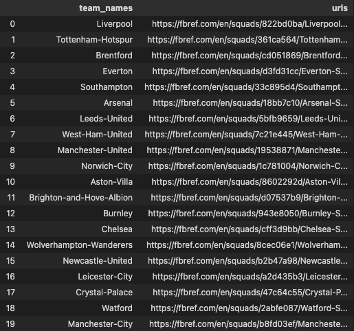
Great start, we can save this dataframe and whenever we want to team level data, we can just query the team name to generate the URL without having to open a web-brower. A further development of this would be to pass a list of the stats pages of all the top 5 leagues to construct a larger data frame that we can save for later. I’m just sticking with the EPL in this example so the code can run quickly.
Let’s now see if we can do the same for players in the same league
Important Functions
As I mentioned before, there are a myriad of pitfalls and issues when I tried to make this and the biggest on was getting the player names to match the URLs. The EPL being the cultural melting pot that it currently exists as today has several players with non ASCII characters in their names. TLDR, loads of players are foreign and have non english standard alphanumeric characters in their names. The following 2 function help us get around that.
Remove accents, converts all the characters of a player name into english standard characters. As these non english characters don’t always relay back to the characters we expect ie; we expect Martin Ødegaard → Martin Odegaard, however we get Martin Ødegaard → Martin Oedegaard. We need to use the fuzzy merge function that acts as a more accurate ‘closest’ match much like using an approximate match on VLOOKUP in MS Excel to ensure we are joining the correct URL to the correct player and further down the line when we query the database we don’t need to worry about totally correct spelling or special characters.
def fuzzy_merge(df_1, df_2, key1, key2, threshold=97, limit=1):
    """
    :param df_1: the left table to join
    :param df_2: the right table to join
    :param key1: key column of the left table
    :param key2: key column of the right table
    :param threshold: how close the matches should be to return a match, based on Levenshtein distance
    :param limit: the amount of matches that will get returned, these are sorted high to low
    :return: dataframe with boths keys and matches
    """
    s = df_2[key2].tolist()

    m = df_1[key1].apply(lambda x: process.extract(x, s, limit=limit))
    df_1['matches'] = m

    m2 = df_1['matches'].apply(lambda x: ', '.join([i[0] for i in x if i[1] >= threshold]))
    df_1['matches'] = m2

    return df_1


def remove_accents(input_str):
    nfkd_form = unicodedata.normalize('NFKD', input_str)
    only_ascii = nfkd_form.encode('ASCII', 'ignore')
    only_ascii = str(only_ascii)
    only_ascii = only_ascii[2:-1]
    only_ascii = only_ascii.replace('-', ' ')
    return only_ascii
Getting Player URLs
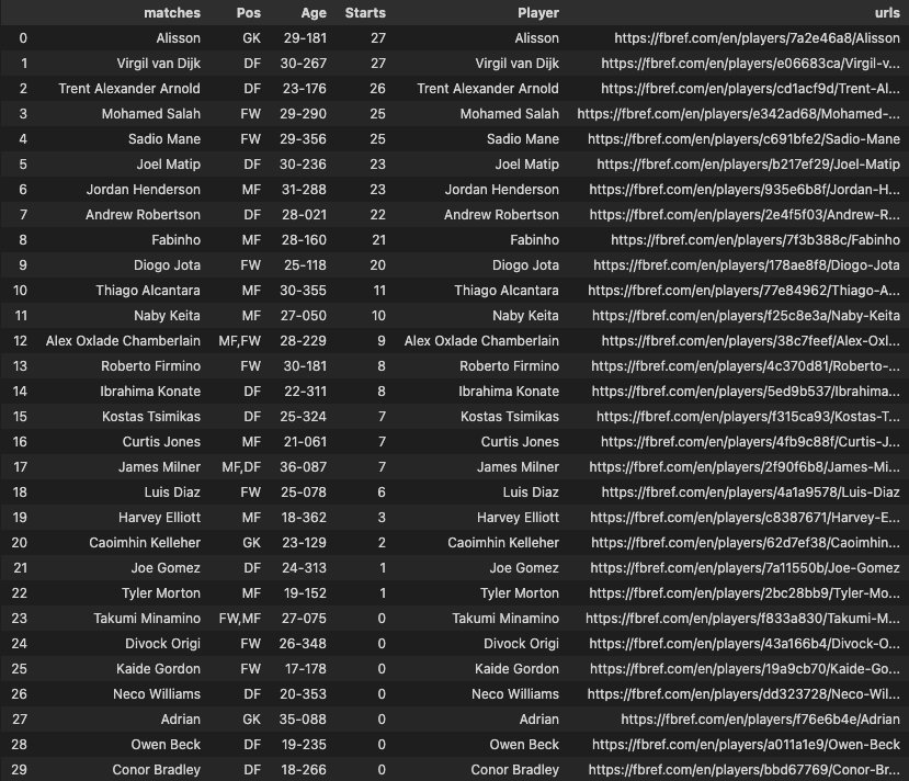
The next functions takes the a list of URLs collated from the get_team_urls() function and builds a new dataframe with the players of all those teams, complete with their Names, Ages & number of starts.
def general_url_database(full_urls):
    appended_data = []
    for team_url in full_urls:
        url = team_url
        player_db = pd.DataFrame()
        player_urls = []
        data  = requests.get(url).text
        links = BeautifulSoup(data).select('th a')
        urls = [link['href'] for link in links]
        player_urls.append(urls)
        player_urls  = [item for sublist in player_urls  for item in sublist]
        player_urls.sort()
        player_urls = list(set(player_urls))
        p_url = list(filter(lambda k: 'players' in k, player_urls))
        url_final = []
        for y in p_url:
            full_url = "https://fbref.com"+y
            url_final.append(full_url)
        player_names = []
        for player in p_url:
            player_name_slice = player[21:]
            player_name_slice = player_name_slice.replace('-', ' ')
            player_names.append(player_name_slice)
        list_of_tuples = list(zip(player_names, url_final))
        play_url_database = pd.DataFrame(list_of_tuples, columns = ['Player', 'urls'])
        player_db = pd.concat([play_url_database])

        html = requests.get(url).text
        data2 = BeautifulSoup(html, 'html5')
        table = data2.find('table')
        cols = []

        for header in table.find_all('th'):
            cols.append(header.string)

        columns = cols[8:37] #gets necessary column headers
        players = cols[37:-2]

        #display(columns)
        rows = [] #initliaze list to store all rows of data
        for rownum, row in enumerate(table.find_all('tr')): #find all rows in table
            if len(row.find_all('td')) > 0:
                rowdata = [] #initiliaze list of row data
                for i in range(0,len(row.find_all('td'))): #get all column values for row
                    rowdata.append(row.find_all('td')[i].text)
                rows.append(rowdata)
        df = pd.DataFrame(rows, columns=columns)

        df.drop(df.tail(2).index,inplace=True)
        df["Player"] = players
        df = df[["Player","Pos","Age", "Starts"]]

        df['Player'] = df.apply(lambda x: remove_accents(x['Player']), axis=1)
        test_merge = fuzzy_merge(df, player_db, 'Player', 'Player', threshold=90)
        test_merge = test_merge.rename(columns={'matches': 'Player', 'Player': 'matches'})
        final_merge = test_merge.merge(player_db, on='Player', how='left')
        appended_data.append(final_merge)
    appended_data = pd.concat(appended_data)
    return appended_data
Data Cleaning
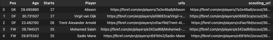
Okay we’re moving in the right direction however, we still need to do some housekeeping to make sure we can query this database easily. Firstly, we need to sort out the ages column, the data seems to constructed in age in years and days format, and more importantly the data type of this column is string so we need to convert that into an integer format.
def years_converter(variable_value):
    years = variable_value[:-4]
    days = variable_value[3:]
    years_value = pd.to_numeric(years)
    days_value = pd.to_numeric(days)
    day_conv = days_value/365
    final_val = years_value + day_conv

    return final_val

EPL_Player_db['Age'] = EPL_Player_db.apply(lambda x: years_converter(x['Age']), axis=1)
EPL_Player_db = EPL_Player_db.drop(columns=['matches'])
Getting detailed scouting report URLs
As I had mentioned previously, one of the issues with scraping FBREF is that there are sub-pages within other sub-pages that are required to access more granular data. However there does exist a page called the 365 Scouting report where hundreds of player metrics are available, in far more detail than just the regular stats page where we have previously explored in part 2. In order to perfrom more detailed analysis, it would make a lot of sense to get all our data from this 365 Scouting report for all players going forward, so we need the option of having this URL at hand.
The issue is again is that URL for this page is again different to that of the parent page.
-
Standard Stats URL: https://fbref.com/en/players/e09f279b/Ivan-Toney
-
Detailed Stats URL: https://fbref.com/en/players/e09f279b/scout/365_euro/Ivan-Toney-Scouting-Report
Luckily there exists a rough pattern with trying to generate the Detailed Stats URL. The following function constructs that URL and appends it on the EPL player database we have just created.
def get_360_scouting_report(url):
    start = url[0:38]+ "scout/365_euro/"
    def remove_first_n_char(org_str, n):
        mod_string = ""
        for i in range(n, len(org_str)):
            mod_string = mod_string + org_str[i]
        return mod_string
    mod_string = remove_first_n_char(url, 38)
    final_string = start+mod_string+"-Scouting-Report"
    return final_string
EPL_Player_db['scouting_url'] = EPL_Player_db.apply(lambda x: get_360_scouting_report(x['urls']), axis=1)
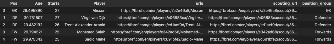
Adding Player Positions
We will be wanting to query this database in future and there are several combinations of player positions in the position columns:
EPL_Player_db.Pos.unique()

array(['GK', 'DF', 'FW,MF', 'FW', 'MF,FW', 'MF', 'MF,DF', 'DF,FW',
       'DF,MF', 'FW,DF'], dtype=object)
In order to easily search through these combinations, I have grouped some of these positions together. The segmentation was decided by me, feel free to edit it if you think it can be refined.
keepers = ['GK']
defenders = ["DF",'DF,MF']
wing_backs = ['FW,DF','DF,FW']
defensive_mids = ['MF,DF']
midfielders = ['MF']
attacking_mids = ['MF,FW',"FW,MF"]
forwards = ['FW']
def position_grouping(x):
    if x in keepers:
        return "GK"
    elif x in defenders:
        return "Defender"
    elif x in wing_backs:
        return "Wing-Back"
    elif x in defensive_mids:
        return "Defensive-Midfielders"
    elif x in midfielders:
        return "Central Midfielders"
    elif x in attacking_mids:
        return "Attacking Midfielders"
    elif x in forwards:
        return "Forwards"
    else:
        return "unidentified position"

EPL_Player_db["position_group"] = EPL_Player_db.Pos.apply(lambda x: position_grouping(x))
Solid, we’ve now got a database of Teams and Players in the EPL that we can easily query and access the detailed and standard metrics from just using their URLs that we have saved.
Lets now perfrom some analysis on population of players in this dataset.
EPL_Player_db.reset_index(drop=True)
EPL_Player_db[["Starts"]] = EPL_Player_db[["Starts"]].apply(pd.to_numeric)
Querying the Database
Arsenal need a Central Midfielder, and badly. It’s my preference that we pick someone young, from the premier league and with minutes under their belt this season.
From my criteria we can set the following filtering parameters:
position = 'Central Midfielders'
pl_starts = 10
max_age = 26

subset_of_data = EPL_Player_db.query('position_group == @position & Starts > @pl_starts & Age < @max_age' )
players_needed = list(subset_of_data.urls.unique())
We’re going to use the get_player_multi_data function written in part two to load all the standard stats of the players in our selected population.
def get_player_multi_data(url_list:list):
appended_data = []
for url in url_list:
warnings.filterwarnings("ignore")
page =requests.get(url)
soup = BeautifulSoup(page.content, 'html.parser')
name = [element.text for element in soup.find_all("span")]
name = name[7]
metric_names = []
metric_values = []
remove_content = ["'", "[", "]", ","]
for row in soup.findAll('table')[0].tbody.findAll('tr'):
first_column = row.findAll('th')[0].contents
metric_names.append(first_column)
for row in soup.findAll('table')[0].tbody.findAll('tr'):
first_column = row.findAll('td')[0].contents
metric_values.append(first_column)
metric_names = [item for sublist in metric_names for item in sublist]
metric_values = [item for sublist in metric_values for item in sublist]
df_player = pd.DataFrame()
df_player['Name'] = name[0]
for item in metric_names:
df_player[item] = []
name = name
non_penalty_goals = (metric_values[0])
npx_g = metric_values[1]
shots_total = metric_values[2]
assists = metric_values[3]
x_a = metric_values[4]
npx_g_plus_x_a = metric_values[5]
shot_creating_actions = metric_values[6]
passes_attempted = metric_values[7]
pass_completion_percent = metric_values[8]
progressive_passes = metric_values[9]
progressive_carries = metric_values[10]
dribbles_completed = metric_values[11]
touches_att_pen = metric_values[12]
progressive_passes_rec = metric_values[13]
pressures = metric_values[14]
tackles = metric_values[15]
interceptions = metric_values[16]
blocks = metric_values[17]
clearances = metric_values[18]
aerials_won = metric_values[19]
df_player.loc[0] = [name, non_penalty_goals, npx_g, shots_total, assists, x_a, npx_g_plus_x_a, shot_creating_actions, passes_attempted, pass_completion_percent,
progressive_passes, progressive_carries, dribbles_completed, touches_att_pen, progressive_passes_rec, pressures, tackles, interceptions, blocks,
clearances, aerials_won]
appended_data.append(df_player)
appended_data = pd.concat(appended_data)
return appended_data
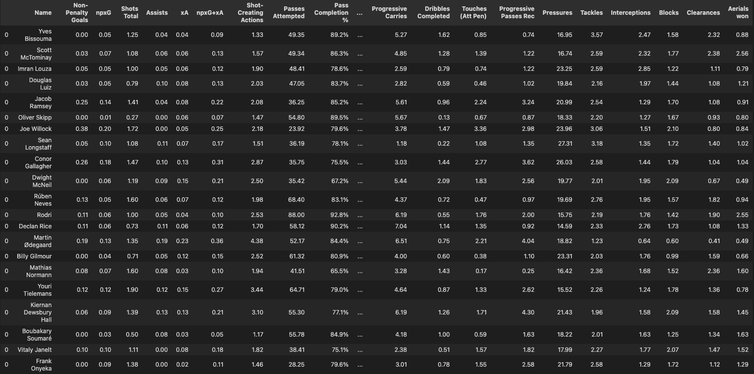
df = get_player_multi_data(players_needed)
EPL Player Progressive Pass Efficeny Chart
In this iteration we have far greater number of players available than just the 4 we manually copied in last time. This allows us to perfrom new types of visualisations, that we previously couldn’t.
Ninad Barbadikar creats some beautiful and insightful charts using tableau, one of which I found quite interesting was his Progressive Passes vs xA per90 scatter plot. I’m going to use the same basis and develop it slightly to meet my data needs.
Again in the case of Arsenal, we are in dire need of a Central Midfielder, to eventually replace Granit Xhaka as Left sided CM. So we’re looking for someone who is not only an very progressive mover of the ball to help us dominante the oppsition in their own defensive 3rd, but we also need a guy who is efficent at making these passes. So I have written a function to plot the Progressive Actions Per 90 vs Number of passes attempted per 90.
I have defined “Progressive_Actions_p90” as ‘Progressive Passes’ + ‘Progressive Carries’. This is to also considers the players who dribble more as well as.
I have shaded a zone in green to illustrate where the elite performers in this metrics exist.
def metrics_scatter_comparison(df, max_age, position):

        df[['Progressive Passes', 'Progressive Carries','Passes Attempted']] =  df[['Progressive Passes','Progressive Carries','Passes Attempted']].apply(pd.to_numeric)
        df["Progressive_Actions_p90"] = df['Progressive Passes'] + df['Progressive Carries']
        df["Passes_Attempted"] = df['Passes Attempted']

        line_color = "silver"

        fig, ax = plt.subplots(figsize=(12, 8))

        ax.scatter(df["Progressive_Actions_p90"], df["Passes_Attempted"],alpha=0.8) ##scatter points
        ax.axvspan(10.0, 14.0, ymin=0.5, ymax=1, alpha=0.1, color='green',label= "In Form")

        texts = [] ##plot player names
        for row in df.itertuples():
                texts.append(ax.text(row.Progressive_Actions_p90, row.Passes_Attempted, row.Name, fontsize=8, ha='center', va='center', zorder=10))
                adjust_text(texts) ## to remove overlaps between labels

        ## update plot
                ax.set(xlabel="Progressive Actions per 90", ylabel="Passes Attempted per 90", ylim=((df["Passes_Attempted"].min()-2), (df["Passes_Attempted"].max()+2)), xlim=((df["Progressive_Actions_p90"].min()-2), (df["Progressive_Actions_p90"].max()+2))) ## set labels and limits

        ##grids and spines
        ax.grid(color=line_color, linestyle='--', linewidth=0.8, alpha=0.5)
        for spine in ["top", "right"]:
                ax.spines[spine].set_visible(False)
                ax.spines[spine].set_color(line_color)

        ax.xaxis.label.set(fontsize=12, fontweight='bold')
        ax.yaxis.label.set(fontsize=12, fontweight='bold') ## increase the weight of the axis labels

        ax.set_position([0.05, 0.05, 0.82, 0.78]) ## make space for the title on top of the axes

        ## title and subtitle
        fig.text(x=0.08, y=0.92, s=f"U-{max_age} {position} | Progressive Actions Profile",
                ha='left', fontsize=20, fontweight='book',
                path_effects=[pe.Stroke(linewidth=3, foreground='0.15'),
                        pe.Normal()])
        fig.text(x=0.08, y=0.88, s=f"EPL | 2021-22", ha='left',
                fontsize=20, fontweight='book',
                path_effects=[pe.Stroke(linewidth=3, foreground='0.15'),
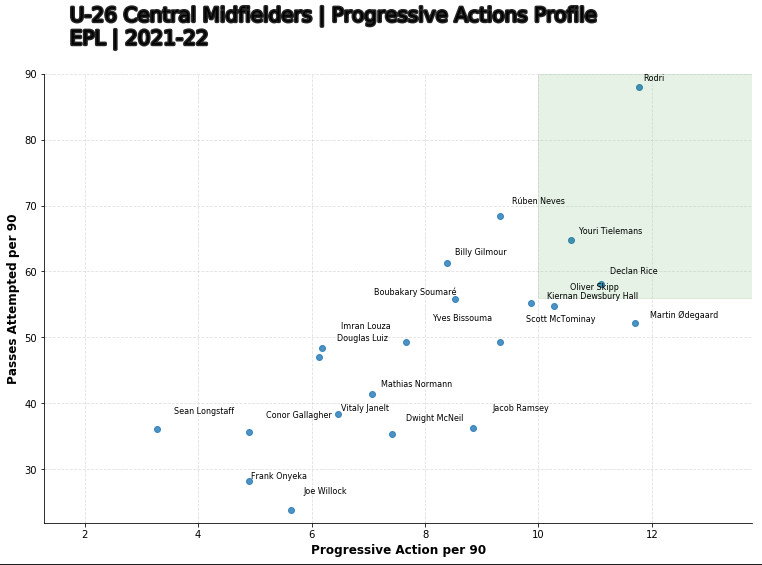
From this chart, we are able to see that, outside of Rodri, Youri Tielemans & Declan Rice, pass at a high volume, but also complete an elite level of progressive action per game among the Central Midifielders in my criteria. Given the recent noise around Declan Rice’s tranfer value being north of £150m, we will not consider him as an option moving forward. A futher development of this database could be to include the a players transfer value to help us narrow down our population.
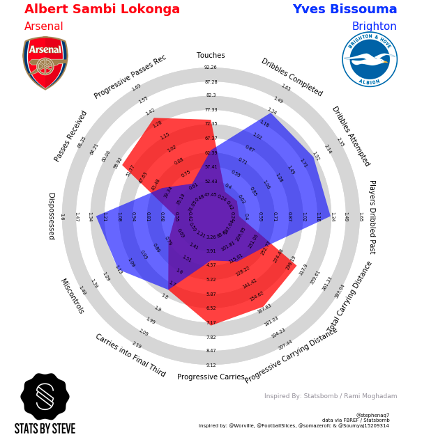
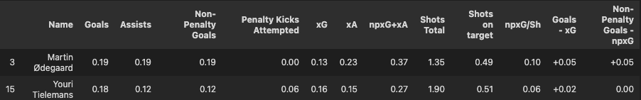
Martin Ødegaard plays the role of the right sided CM in Arsenal’s system and we’re looking a player to fill the left sided role. As both sides of the CM position need to perform similar tasks, it would be wise to compare the potential player to MØ So lets see how Youri shapes up against MØ.
We’re going to retrieve the Detailed Stats for both players, scraping their advanced stats page from the URLs we saved earlier. The following function will create a dataframe comprising all the metrics for both players.
Loading Advanced Scouting Data
scout_links = list(subset_of_data.scouting_url.unique())
def generate_advanced_data(scout_links):
    appended_data_per90 = []
    appended_data_percent = []
    for x in scout_links:
        warnings.filterwarnings("ignore")
        url = x
        page =requests.get(url)
        soup = BeautifulSoup(page.content, 'html.parser')
        name = [element.text for element in soup.find_all("span")]
        name = name[7]
        html_content = requests.get(url).text.replace('<!--', '').replace('-->', '')
        df = pd.read_html(html_content)
        df[0].columns = df[0].columns.droplevel(0) # drop top header row
        stats = df[0]
        advanced_stats = stats.loc[(stats['Statistic'] != "Statistic" ) & (stats['Statistic'] != ' ')]
        advanced_stats = advanced_stats.dropna(subset=['Statistic',"Per 90", "Percentile"])
        per_90_df = advanced_stats[['Statistic',"Per 90",]].set_index("Statistic").T
        per_90_df["Name"] = name
        percentile_df = advanced_stats[['Statistic',"Percentile",]].set_index("Statistic").T
        percentile_df["Name"] = name
        appended_data_per90.append(per_90_df)
    appended_data_per90 = pd.concat(appended_data_per90)
    appended_data_per90 = appended_data_per90.reset_index(drop=True)
    del appended_data_per90.columns.name
    appended_data_per90 = appended_data_per90[['Name'] + [col for col in appended_data_per90.columns if col != 'Name']]
    appended_data_per90 = appended_data_per90.loc[:,~appended_data_per90.columns.duplicated()]
    return appended_data_per90
As we now have all the stats needed for the players, 120 in total, it’s best to catergorise them. The snippet below shows how I’ve grouped all the stats together. I have tried to keep as close to what is used in FBREF but with some slight changes.
attacking = ["Name",'Goals', 'Assists', 'Non-Penalty Goals','Penalty Kicks Attempted', 'xG',
      'xA', 'npxG+xA', 'Shots Total', 'Shots on target', 'npxG/Sh',
       'Goals - xG', 'Non-Penalty Goals - npxG']
passing = ["Name", 'Passes Completed','Passes Attempted', 'Pass Completion %', 'Total Passing Distance',
       'Progressive Passing Distance', 'Passes Completed (Short)',
       'Passes Attempted (Short)', 'Pass Completion % (Short)',
       'Passes Completed (Medium)', 'Passes Attempted (Medium)',
       'Pass Completion % (Medium)', 'Passes Completed (Long)',
       'Passes Attempted (Long)', 'Pass Completion % (Long)',
       'Key Passes', 'Passes into Final Third',
       'Passes into Penalty Area', 'Crosses into Penalty Area',
       'Progressive Passes']
pass_types = ["Name", 'Live-ball passes', 'Dead-ball passes',
       'Passes from Free Kicks', 'Through Balls', 'Passes Under Pressure',
       'Switches', 'Crosses', 'Corner Kicks', 'Inswinging Corner Kicks',
       'Outswinging Corner Kicks', 'Straight Corner Kicks',
       'Ground passes', 'Low Passes', 'High Passes',
       'Passes Attempted (Left)', 'Passes Attempted (Right)',
       'Passes Attempted (Head)', 'Throw-Ins taken',
       'Passes Attempted (Other)', 'Passes Offside',
       'Passes Out of Bounds', 'Passes Intercepted', 'Passes Blocked']
chance_creation = ["Name",'Shot-Creating Actions', 'SCA (PassLive)', 'SCA (PassDead)',
       'SCA (Drib)', 'SCA (Sh)', 'SCA (Fld)', 'SCA (Def)',
       'Goal-Creating Actions', 'GCA (PassLive)', 'GCA (PassDead)',
       'GCA (Drib)', 'GCA (Sh)', 'GCA (Fld)', 'GCA (Def)']
defending = [ "Name", 'Tackles',
       'Tackles Won', 'Tackles (Def 3rd)', 'Tackles (Mid 3rd)',
       'Tackles (Att 3rd)', 'Dribblers Tackled', 'Dribbles Contested', 'Dribbled Past', 'Pressures',
       'Successful Pressures', 'Successful Pressure %',
       'Pressures (Def 3rd)', 'Pressures (Mid 3rd)',
       'Pressures (Att 3rd)', 'Blocks', 'Shots Blocked', 'Shots Saved',
       'Interceptions', 'Tkl+Int', 'Clearances', 'Errors','Ball Recoveries',
       'Aerials won', 'Aerials lost']
possesion = ["Name", 'Touches',
       'Touches (Def Pen)', 'Touches (Def 3rd)', 'Touches (Mid 3rd)',
       'Touches (Att 3rd)', 'Touches (Att Pen)', 'Touches (Live-Ball)',
       'Dribbles Completed', 'Dribbles Attempted', 'Successful Dribble %',
       'Players Dribbled Past', 'Nutmegs', 'Carries',
       'Total Carrying Distance', 'Progressive Carrying Distance',
       'Progressive Carries', 'Carries into Final Third',
       'Carries into Penalty Area', 'Miscontrols', 'Dispossessed',
       'Pass Targets', 'Passes Received', 'Passes Received %',
       'Progressive Passes Rec']
dicipline = ["Name", 'Yellow Cards', 'Red Cards','Second Yellow Card', 'Fouls Committed','Offsides','Penalty Kicks Conceded', 'Own Goals']
smarts = ["Name",'Penalty Kicks Won','Fouls Drawn']
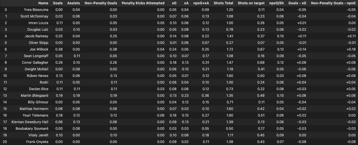
Now that we have categorised our metrics let’s take a look at their attacking numbers.
per_90_dataframe = appended_data_per90[attacking]
per_90_dataframe
Improved Radar Chart
In part 2, we went through the basics of how to generate a radar diagrams and the pros and cons of using one. Now that we have a more complere set of metrics, I’m going to use a slightly different template for the plots. The Radar package from Soccerplots give’s us a clean chart & customisable chart, where we can plot all the per 90 metrics without having to transform the data or use percentile metrics like we did in part 2.
names = ["Youri Tielemans","Martin Ødegaard"]
per_90_dataframe = per_90_dataframe[per_90_dataframe.Name.isin(names)]
player_names = list(per_90_dataframe.Name.unique())
per_90_dataframe.reset_index(drop=True)
per_90_dataframe = per_90_dataframe[per_90_dataframe.Name.isin(names)]
cols = per_90_dataframe.columns.drop('Name')
per_90_dataframe[cols] = per_90_dataframe[cols].apply(pd.to_numeric)
params = list(per_90_dataframe.columns)
params = params[1:]
params

ranges = []
a_values = []
b_values = []

for x in params:
    a = min(per_90_dataframe[params][x])
    a = a - (a* 0.25)

    b = max(per_90_dataframe[params][x])
    b = b + (b* 0.25)

    ranges.append((a,b))

a_values = per_90_dataframe.iloc[0].values.tolist()

b_values = per_90_dataframe.iloc[1].values.tolist()

a_values = a_values[1:]
b_values = b_values[1:]

values = [a_values,b_values]

get_clubs = subset_of_data[subset_of_data.Player.isin(names)]
link_list = list(get_clubs.urls.unique())
title_vars = []
for x in link_list:
    warnings.filterwarnings("ignore")
    html_content = requests.get(x).text.replace('<!--', '').replace('-->', '')
    df2 = pd.read_html(html_content)
    df2[5].columns = df2[5].columns.droplevel(0)
    stats2 = df2[5]
    key_vars = stats2[["Season","Age","Squad"]]
    key_vars = key_vars[key_vars.Season.isin(["2021-2022"])]
    title_vars.append(key_vars)
title_vars = pd.concat(title_vars)
ages = list(title_vars.Age.unique())
teams = list(title_vars.Squad.unique())

#title

title = dict(
    title_name= player_names[0],
    title_color = 'red',
    subtitle_name = teams[0],
    subtitle_color = 'red',

    title_name_2= player_names[1],
    title_color_2 = 'blue',
    subtitle_name_2 = teams[1],
    subtitle_color_2 = 'blue',
    title_fontsize = 18,
    subtitle_fontsize=15
)

endnote = '@stephenaq7\ndata via FBREF / Statsbomb'

radar = Radar()

fig,ax = radar.plot_radar(ranges=ranges,params=params,values=values,
                         radar_color=['red','blue'],
                         alphas=[.75,.6],title=title,endnote=endnote,
                         compare=True)
We should get this following output:
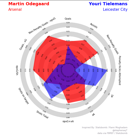
Excellent, we now have a cleaner radar plot, where each metrics is normalised to their own scale and we can now add more information to the charts such as the team.
Conclusion
From the objectives we set out, we needed to:
- Build a method to programaticaly access player & team level data with minimal input
We have managed to do this, we have built a database of player & team URLs to easily access data from FBREF and use those metrics to do some basic data analysis.
I will be building more functions to make the access of data slightly smoother and will be creating more visuals similar to the progressive pass chart to look for some interesting correlations between positions and other metrics.
I hope you learned something from these posts and if you feel like I’ve missed out some glaring holes or have any other suggestions then please feel free to reach out to me
Thanks for reading,
Steve

Comments