26 min to read
FBREF Data Scraping Walk Through pt2
Advanced techniques for scraping football data from FBREF
In part one of the data scraping walk through, we successfully achieved the following items;
-
Create a set of working functions to aggregate data from FBREF.
-
Perform a series of data munging tasks to get easy to to use datasets ready for analysis.
-
Create a series of Data Visualisations from these cleaned datasets.
Although there is still one action not currently explored:
- Assess the meaningful metrics we need to start making some predictions on player suitability to positions.
We have not yet aquired any player level data. This post will outline the methods by which player level performance data can be webscraped from FBREF.com and how to use that information to compare player metrics. Some of the code in this post has been repurposed from this great article from Frank Hopkins on how to scrape data from FBREF in order to compare players.
Code and notebook for this post can be found here.
Setup
First up, we import all our necessary packages for web-scraping, data cleaning and analysis.
import requests
import pandas as pd
from bs4 import BeautifulSoup
import seaborn as sb
import matplotlib.pyplot as plt
import matplotlib as mpl
import warnings
import numpy as np
from math import pi
Data
In my last post, I picked Napoli as the team to analyse, but since we’re looking at players now, I’m going to keep it #Brexit, and have a look at the young up and coming, English attacking midfield players currently in the EPL.
To narrow it down I’ve gone with U23 players, so in no particular order:
England Star Boy Analysis


Getting player data from the FBREF Sub-pages.
For the full code visit my repo.
The first function requires the URL of a player profile to be passed in order to return a pandas dataframe with the high level per/90 stats available on this page. The beautiful soup package will find the tables we need in the source code of the html. The table we want from this sub-page is structured slightly differently to the one we have scraped previously. So we need to construct our dataframe in a more programmatic way.
def get_player_data(x):
    warnings.filterwarnings("ignore")
    url = x
    page =requests.get(url)
    soup = BeautifulSoup(page.content, 'html.parser')
    name = [element.text for element in soup.find_all("span")]
    name = name[7]
    metric_names = []
    metric_values = []
    for row in soup.findAll('table')[0].tbody.findAll('tr'):
        first_column = row.findAll('th')[0].contents
        metric_names.append(first_column)
    for row in soup.findAll('table')[0].tbody.findAll('tr'):
        first_column = row.findAll('td')[0].contents
        metric_values.append(first_column)

    metric_names = [item for sublist in metric_names for item in sublist]
    metric_values = [item for sublist in metric_values for item in sublist]
    df_player = pd.DataFrame()
    df_player['Name'] = name[0]
    for item in metric_names:
        df_player[item] = []

    name = name
    non_penalty_goals = (metric_values[0])
    npx_g = metric_values[1]
    shots_total = metric_values[2]
    assists = metric_values[3]
    x_a = metric_values[4]
    npx_g_plus_x_a = metric_values[5]
    shot_creating_actions = metric_values[6]
    passes_attempted = metric_values[7]
    pass_completion_percent = metric_values[8]
    progressive_passes = metric_values[9]
    progressive_carries = metric_values[10]
    dribbles_completed = metric_values[11]
    touches_att_pen = metric_values[12]
    progressive_passes_rec = metric_values[13]
    pressures = metric_values[14]
    tackles = metric_values[15]
    interceptions = metric_values[16]
    blocks = metric_values[17]
    clearances = metric_values[18]
    aerials_won = metric_values[19]
    df_player.loc[0] = [name, non_penalty_goals, npx_g, shots_total, assists, x_a, npx_g_plus_x_a, shot_creating_actions, passes_attempted, pass_completion_percent,
                        progressive_passes, progressive_carries, dribbles_completed, touches_att_pen, progressive_passes_rec, pressures, tackles, interceptions, blocks,
                        clearances, aerials_won]
    return df_player
Comparing Player Metrics
The above functions works on any page with this template so effectively any teams stats page will work with this..hopefully. I’m probably one of the most insufferable Arsenal fans you’ll ever meet so in typical fashion I’ve gone with, Bukayo Saka, who in my opinion is going to outdo Henry’s legacy.
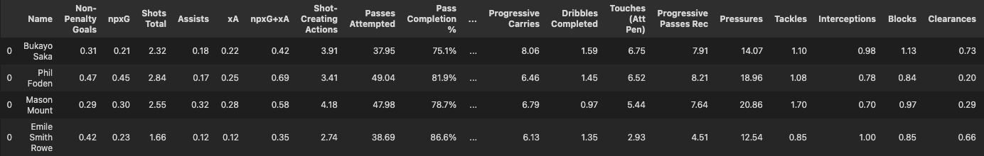
get_player_data("https://fbref.com/en/players/bc7dc64d/Bukayo-Saka")
Now lets have a look a the output:

This is okay but, its only one player using one URL, in the next function we will pass a list of URLs instead and generate an dataframe with the stats of multiple players. Let now get all the stats of players selected for the analysis in one dataframe.
url_list = ["https://fbref.com/en/players/bc7dc64d/Bukayo-Saka","https://fbref.com/en/players/ed1e53f3/Phil-Foden","https://fbref.com/en/players/9674002f/Mason-Mount","https://fbref.com/en/players/17695062/Emile-Smith-Rowe"]

get_player_multi_data(url_list)
This is in much better shape now, there is still some data cleaning to do however, after we have sorted that, we can start creating some visuals to make it it easier to compare the players.
As you may have noticed from the output table, we have a lot of features in our dataframe. Luckily we can group some of these into categories. In order to keep thing simple, I went with using - ‘Attacking’, ‘Playmaking’, & ‘Defensive’ as the categories. The features selected for each one have been chose using the same grouping in FBREF.
def generate_player_comparison(url_list, view):
    df_player_comp = get_player_multi_data(url_list)

    def p2f(x):
        return float(x.strip('%'))/100

    df_player_comp["Pass Completion %"] = df_player_comp["Pass Completion %"].apply(p2f)

    df_player_comp[['Non-Penalty Goals', 'npxG', 'Shots Total', 'Assists', 'xA',
        'npxG+xA', 'Shot-Creating Actions', 'Passes Attempted',
        'Pass Completion %', 'Progressive Passes', 'Progressive Carries',
        'Dribbles Completed', 'Touches (Att Pen)', 'Progressive Passes Rec',
        'Pressures', 'Tackles', 'Interceptions', 'Blocks', 'Clearances',
        'Aerials won']] = df_player_comp[['Non-Penalty Goals', 'npxG', 'Shots Total', 'Assists', 'xA',
        'npxG+xA', 'Shot-Creating Actions', 'Passes Attempted',
        'Pass Completion %', 'Progressive Passes', 'Progressive Carries',
        'Dribbles Completed', 'Touches (Att Pen)', 'Progressive Passes Rec',
        'Pressures', 'Tackles', 'Interceptions', 'Blocks', 'Clearances',
        'Aerials won']].apply(pd.to_numeric)

    df_player_comp_attacking= df_player_comp[['Name','Non-Penalty Goals', 'npxG', 'Shots Total','xA','npxG+xA', 'Shot-Creating Actions']]

    df_player_comp_playmaking= df_player_comp[['Name','Assists','Dribbles Completed',
         'Touches (Att Pen)', 'Progressive Passes Rec','Passes Attempted',
        'Pass Completion %', 'Progressive Passes', 'Progressive Carries']]

    df_player_comp_defensive= df_player_comp[['Name','Aerials won','Pressures', 'Tackles', 'Interceptions', 'Blocks']]

    if view == "attack":
        fig, ax =plt.subplots(1,3, figsize=(27,6))
        sb.barplot(df_player_comp_attacking['Name'], df_player_comp_attacking['Non-Penalty Goals'], ax=ax[0]).set(title='Non Penalty Goals')
        sb.barplot(df_player_comp_attacking['Name'], df_player_comp_attacking['npxG'], ax=ax[1]).set(title='Non Penalty xG')
        sb.barplot(df_player_comp_attacking['Name'], df_player_comp_attacking['Shots Total'], ax=ax[2]).set(title='Total Shots')
    elif view == "playmaking":
        fig, ax =plt.subplots(1,4, figsize=(27,6))
        sb.barplot(df_player_comp_playmaking['Name'], df_player_comp_playmaking['Assists'], ax=ax[0]).set(title='Assists')
        sb.barplot(df_player_comp_playmaking['Name'], df_player_comp_playmaking['Dribbles Completed'], ax=ax[1]).set(title='Dribbles Completed')
        sb.barplot(df_player_comp_playmaking['Name'], df_player_comp_playmaking['Touches (Att Pen)'], ax=ax[2]).set(title='Touches in Pen Area')
        sb.barplot(df_player_comp_playmaking['Name'], df_player_comp_playmaking['Progressive Passes Rec'], ax=ax[3]).set(title='Progressive Passes Received')
    elif view == "defensive":
        fig, ax =plt.subplots(1,5, figsize=(36,8))
        sb.barplot(df_player_comp_defensive['Name'], df_player_comp_defensive['Aerials won'], ax=ax[0]).set(title='Aerials Won')
        sb.barplot(df_player_comp_defensive['Name'], df_player_comp_defensive['Pressures'], ax=ax[1]).set(title='Pressures')
        sb.barplot(df_player_comp_defensive['Name'], df_player_comp_defensive['Tackles'], ax=ax[2]).set(title='Tackles')
        sb.barplot(df_player_comp_defensive['Name'], df_player_comp_defensive['Interceptions'], ax=ax[3]).set(title='Interceptions')
        sb.barplot(df_player_comp_defensive['Name'], df_player_comp_defensive['Blocks'], ax=ax[4]).set(title='Blocks')
    else:
        print('Please check your spelling. options are: attack, playmaking or defensive')
generate_player_comparison(url_list, "attack")
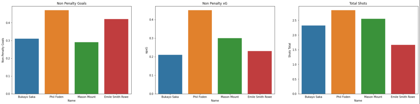
To absolutely nobody’s surprise, Phil Foden tops out all the attacking metircs that we’ve selected. Now, that probably because out of all the players selected, he probably plays most of his football in an advanced ‘false 9’ role, however its still mighty impressive at his age, he’s producing an elite level of output. His npxG (no penalty expected goals) per 90 is in the 97th percentile against wingers & attacking midfielders in europes top 5 leagues. Impressive. The other boy’s aren’t slouches either, putting up impressive attacking numbers.
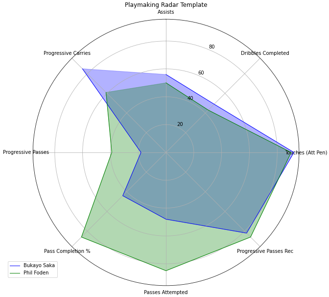
generate_player_comparison(url_list, "playmaking")
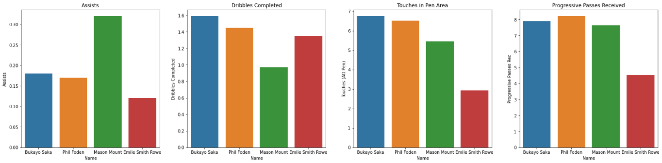
In the playmaking department, my boy Bukayo shares the crown with Mason Mount. Saka is clearly the better dribbler and the most active in the opposition penalty area in terms of touches. Mount tops the Shot-creating actions and Assists metrics, however this is to be expected expected as Mount is the only true #10 on this current roster.
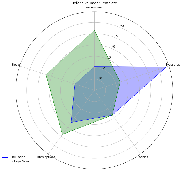
generate_player_comparison(url_list, "defensive")
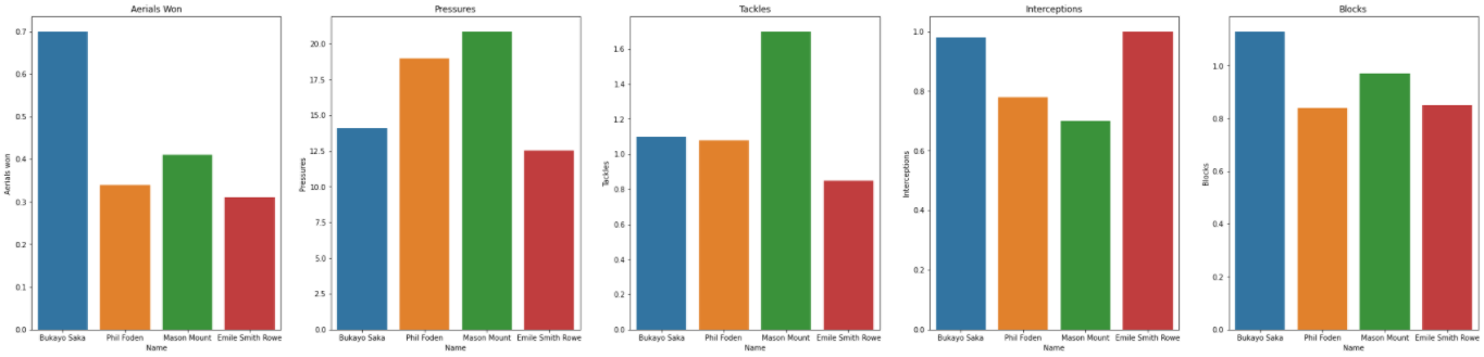
Lastly lets have look at the defensive end of the game, often a forgotten side to evaluate when assessing attacking players. Saka again leads the pack in terms of Aerials won & blocks, and also coming second to his Arsenal Compatriot Emile Smith Rowe for Interceptions. Mason Mount however appears to be the more accomplished tackler and presser of the group. Given the role he plays at Chelsea and the system that is defensively minded this is to be expected.
Fantastic, we’ve managed to collate the data of several players at once using only the URLs of each players stats page in FBREF. We have also managed to utilise some basic matplotlib functions to generate some useful charts.
Developing more intuitive Data Visualisations
Bar charts are useful for comparing players but what if wanted to to view multiple player attributes at once that may overlap the categories that have already been pre determined by me. What if the number of features we want to compare become variable, we would need to edit the subplots every time or develop a more complex function for a chart that doesn’t really tell us that much.
That where Radar plots come in. Radar plots allow us to visually represent one or more groups of values over multiple identically scaled variables.
Creating Radar-Plots with Matplotlib
Why use Radar/Spider Diagrams

- Radar charts are excellent for visualizing comparisons between observations — you can easily compare multiple attributes among different observations and see how they stack up. For example, you could use radar charts to compare restaurants based on some common variables.
- It’s easy to see overall “top performers” — the observation with the highest polygon area should be the best if you’re looking at the overall performance.
However these reasons to use come with their own drawbacks, some which being;
- Radar charts can get confusing fast — comparing more than a handful of observations leads to a mess no one wants to look at.
- It can be tough to find the best options if there are too many variables — just imagine seeing a radar chart with 20+ variables. No one wants to even look at it; God forbid to interpret it.
- The variables have to be on the same scale — it makes no sense to compare student grades (ranging from 1 to 5) and satisfaction with some service (ranging from 0 to 100).
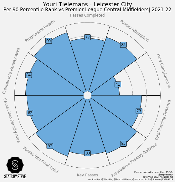
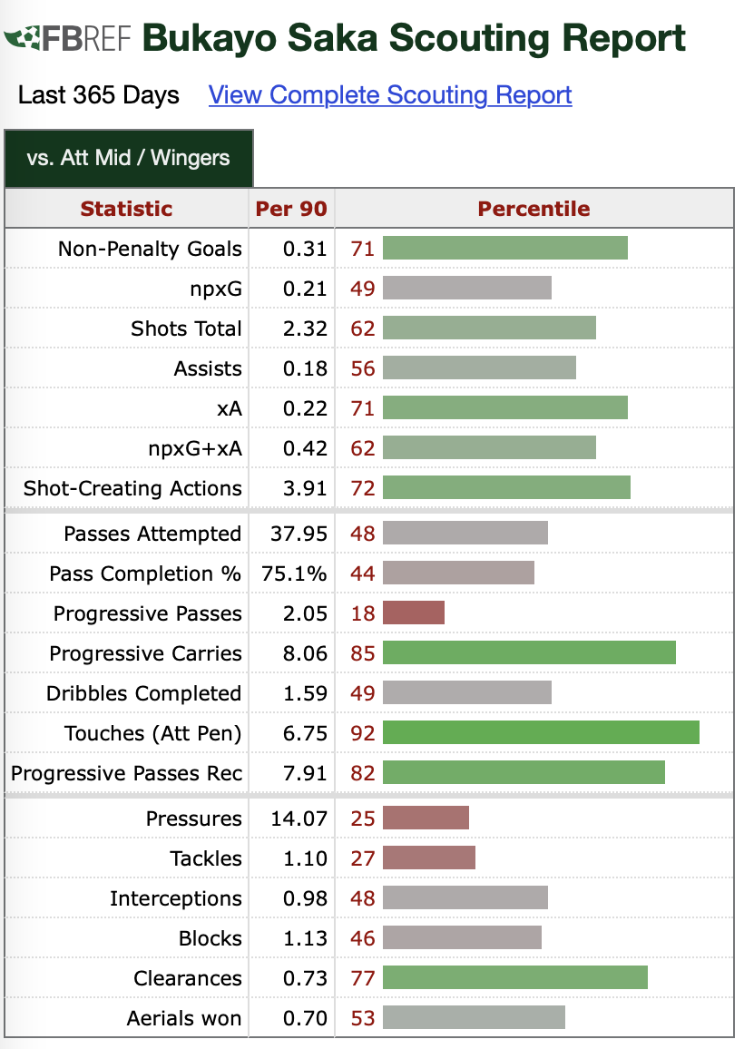
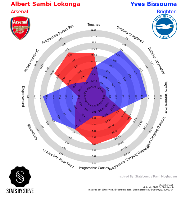
Luckily, we’re able to circumvent these issues without having to transform the data we’re trying to extrapolate insights from. Remember the player data in FBREF, come in 2 formats. ‘Per-90’ & ‘percentile’. The percentile stats offer us a way to normalise all the metrics and in addition they offer their own discrete method of comparison of how a given players metrics measure up to other players in their position/role. In the screen grab below, you will be able to see how the FBREF sub-page displasy this information
In the following function, compare_players_percentile function, accepts two FBRef player urls and compares them in terms of the percentile they fall in for a given metric.
To start with lets pass Foden’s and Saka’s URLs through the function.
def compare_players_percentile(x):
    appended_data = []
    for x in url_list:

        warnings.filterwarnings("ignore")

        url = x
        page =requests.get(url)
        soup= BeautifulSoup(page.content, 'html.parser')
        name = [element.text for element in soup.find_all("span")]
        name = name[7]

        metric_names = []
        metric_values = []


        for row in soup.findAll('table')[0].tbody.findAll('tr'):
            first_column = row.findAll('th')[0].contents
            metric_names.append(first_column)


        for row in soup.findAll('table')[0].tbody.findAll('tr'):
            first_column = row.findAll('td')[1].contents
            metric_values.append(first_column)


        clean_left = []
        splitat_r = 65
        splitat_l = 67

        for item in metric_values:
            item = str(item).strip('[]')
            left, right = item[:splitat_l], item[splitat_r:]
            clean_left.append(left)

        clean_overall= []

        for item in clean_left:
            item = str(item).strip('[]')
            left, right = item[:splitat_l], item[splitat_r:]
            clean_overall.append(right)

        clean = []

        for item in clean_overall:
            item = item.replace("<","")
            clean.append(item)

        metric_names  = [item for sublist in metric_names  for item in sublist]

        clean = list(filter(None, clean))


        df_player = pd.DataFrame()


        df_player['Name'] = name[0]
        for item in metric_names:
            df_player[item] = []


        name = name
        non_penalty_goals = (clean[0])
        npx_g = clean[1]
        shots_total = clean[2]
        assists = clean[3]
        x_a = clean[4]
        npx_g_plus_x_a = clean[5]
        shot_creating_actions = clean[6]
        passes_attempted = clean[7]
        pass_completion_percent = clean[8]
        progressive_passes = clean[9]
        progressive_carries = clean[10]
        dribbles_completed = clean[11]
        touches_att_pen = clean[12]
        progressive_passes_rec = clean[13]
        pressures = clean[14]
        tackles = clean[15]
        interceptions = clean[16]
        blocks = clean[17]
        clearances = clean[18]
        aerials_won = clean[19]
        df_player.loc[0] = [name, non_penalty_goals, npx_g, shots_total, assists, x_a, npx_g_plus_x_a, shot_creating_actions, passes_attempted, pass_completion_percent,
                            progressive_passes, progressive_carries, dribbles_completed, touches_att_pen, progressive_passes_rec, pressures, tackles, interceptions, blocks,
                            clearances, aerials_won]
        appended_data.append(df_player)

    df_player_comp = pd.concat(appended_data)

    df_player_comp[['Non-Penalty Goals', 'npxG', 'Shots Total', 'Assists', 'xA',
            'npxG+xA', 'Shot-Creating Actions', 'Passes Attempted',
            'Pass Completion %', 'Progressive Passes', 'Progressive Carries',
            'Dribbles Completed', 'Touches (Att Pen)', 'Progressive Passes Rec',
            'Pressures', 'Tackles', 'Interceptions', 'Blocks', 'Clearances',
            'Aerials won']] = df_player_comp[['Non-Penalty Goals', 'npxG', 'Shots Total', 'Assists', 'xA',
            'npxG+xA', 'Shot-Creating Actions', 'Passes Attempted',
            'Pass Completion %', 'Progressive Passes', 'Progressive Carries',
            'Dribbles Completed', 'Touches (Att Pen)', 'Progressive Passes Rec',
            'Pressures', 'Tackles', 'Interceptions', 'Blocks', 'Clearances',
            'Aerials won']].apply(pd.to_numeric)

    categories = ['Non-Penalty Goals', 'npxG', 'Shots Total', 'Assists', 'xA',
        'npxG+xA', 'Shot-Creating Actions', 'Passes Attempted',
        'Pass Completion %', 'Progressive Passes', 'Progressive Carries',
        'Dribbles Completed', 'Touches (Att Pen)', 'Progressive Passes Rec',
        'Pressures', 'Tackles', 'Interceptions', 'Blocks', 'Clearances',
        'Aerials won']


    df_player_plot_1 = df_player_comp.reset_index(drop=True)

    df_player_plot_1 = df_player_plot_1.iloc[0].values.tolist()
    player_1_name = df_player_plot_1[0]
    del df_player_plot_1[0]

    df_player_plot_2 = df_player_comp.reset_index(drop=True)
    df_player_plot_2 = df_player_plot_2.iloc[1].values.tolist()
    player_2_name = df_player_plot_2[0]
    del df_player_plot_2[0]

    df_player_1_plot = df_player_plot_1

    df_player_2_plot = df_player_plot_2

    df_player_1_plot_numeric = []

    for item in df_player_1_plot:
        item = int(item)
        df_player_1_plot_numeric.append(item)

    df_player_2_plot_numeric = []

    for item in df_player_2_plot:
        item = int(item)
        df_player_2_plot_numeric.append(item)

    N = 20

    angles = [n / float(N) * 2 * pi for n in range(N)]

    plt.figure(figsize=(40,10))

    ax = plt.subplot(111, polar=True)

    ax.set_theta_offset(pi / 2)

    ax.set_theta_direction(-1)

    plt.xticks(angles[:], categories)

    a = df_player_1_plot_numeric
    b = df_player_2_plot_numeric

    ax.plot(angles, a, linewidth=1, linestyle='solid', label=player_1_name, color ='blue')
    ax.fill(angles, a, 'b', alpha=0.3, color ='blue')

    ax.plot(angles, b, linewidth=1, linestyle='solid', label=player_2_name, color ='green')
    ax.fill(angles, b, 'b', alpha=0.3, color ='green')

    plt.legend(loc='upper right', bbox_to_anchor=(0.1, 0.1))
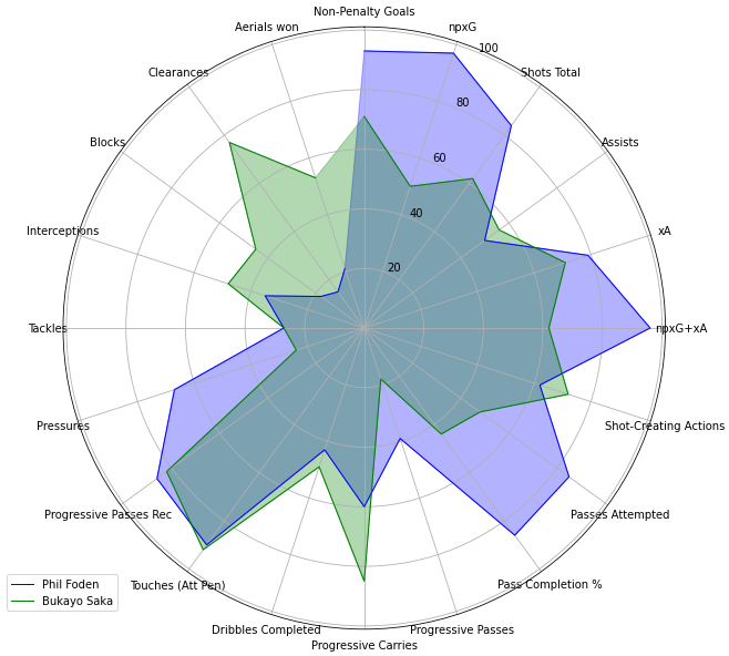
Here, we now have a visulisation that can be extremely insightful for comparing platers of a similar position and hence helping us start to answer which metrics are going to be useful to make some predictions on player position suitability. We can use charts like this to infer the attributes that are more or less important for any given position. In this example, we can see that it can be seen above that despite leading in several attacking metrics, Foden exists in a very low percentile for a number of defensive attributes, whilst Saka appears to be a more rounded player. Now of course these players play the attacking midfield/forward roles with different instuctions and in different formation systems, but seeing as we are also assessing which percentile they exist in compared to the entire FBRef database, this is incredibly useful information. We can conclude without much doubt that the resounding winner of our ‘England Star-Boy’ analysis is Phil Foden.
–page-break–
Attribute Specific Radar-Plots
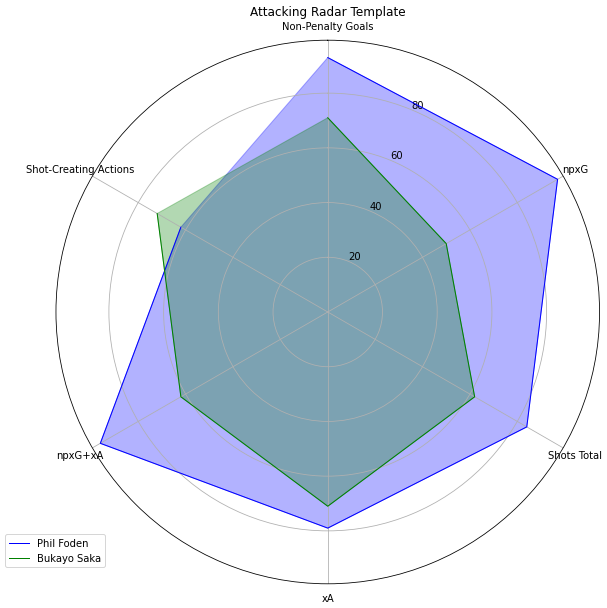
Now lets take things a step further and create the same plots but with a variable number of features, similar to what we did with the bar charts. We will create an attacking, playmaking and defensive template. The code for this function is extremely dense as its been written in a for-loop so for the full code please visit my repo.
Utilising this method of creating intuitive charts with a variable number of metrics we’re trying to compare can help us drill down on which attributes are more important for a given positions. In addition it would help to this type of function if we would want to include less or more attributes when comparing players without having to re write the function every time we want to make changes.
compare_players_percentile_template(url_list,"Attacking")
compare_players_percentile_template(url_list,"Playmaking")
compare_players_percentile_template(url_list,"Defensive")
Conclusion
From the objectives we set out, we needed to gather player data from FBREF using a webscraper, in order to:
- Assess the meaningful metrics we need to start making some predictions on player suitability to positions.
We have managed to do so, and through employing more advanced data visualisation techniques, we are able to infer the performance level of any given player and compare like for like metrics with not only the players in question but also how they compare to other elite players in the FBREF database as well.
Webscraping has proved to be a useful way of circumventing the problematic mnature of finding data for a sports analytics task. The Beautiful Soup Python library, does the majority of the heavy lifting for you when scanning a website for useful information.
However accessing player and team URLs is still a clunky process that requires me to search for the page on web-browers and copy the link over to my notebooks. In order to make any more significant in-roads outside of making some nice charts, the scale of analysis has to increase and the current methods I have used are not seemless enough. So I’ve decided to add another action that we will explore, which is to:
- Build a method to programaticaly access player & team level data with minimal input
Next week we’re going to be creating our own database of player data or create a means to easily access the data of multiple players at once.
Thanks for reading!
Steve

Comments