39 min to read
Exploring mplsoccer - Advanced Player Analysis
Exploring mplsoccer data visualisation
This post is part of a series of how tos for creating dynamic & repeatable functions that are able to produce informative data visualisations for social media or just generally for fun.
Armed with both the Beautiful Soup & mplsoccer python modules I will outline how I do so for my twitter and bluesky posts.
For this instance we’ll be focusing on creating individual and comparison pizza plots using percentile rank statistics from FBREF.
Setup
Here are some of the key modules that are required in order to run this script. This code imports several Python libraries, including requests, json, seaborn, pandas, and more, to support various data processing and visualization tasks. It also utilizes specific tools like MobFot for mobile image recognition, fuzzywuzzy for string matching, and mplsoccer for pizza charts. Additionally, it configures the plotting style to ‘fivethirtyeight’ for a consistent visual theme throughout the analysis.
import requests
import json
from mobfot import MobFot
import unicodedata
from fuzzywuzzy import fuzz
from fuzzywuzzy import process
import seaborn as sb
import pandas as pd
import matplotlib.pyplot as plt
import matplotlib.cbook as cbook
import matplotlib.image as image
import matplotlib.style as style
import matplotlib as mpl
import matplotlib.patheffects as pe
import warnings
import os
import numpy as np
from math import pi
from bs4 import BeautifulSoup
from urllib.request import urlopen
from highlight_text import fig_text
from adjustText import adjust_text
from soccerplots.radar_chart import Radar
from mplsoccer import PyPizza, add_image, FontManager

style.use('fivethirtyeight')
Data Preparation & Constructing Functions
In order to ensure we are able to retrieve the plots we want with ease at a later stage its important that we build out a few function to make things easier down the line. The data we’re going scrape has a lot of inconsistencies with data-types, data-formats and even fonts & characters. The functions below handle many of the most tricky issues regarding data processes.
def fuzzy_merge(df_1, df_2, key1, key2, threshold=97, limit=1):
    """
    :param df_1: the left table to join
    :param df_2: the right table to join
    :param key1: key column of the left table
    :param key2: key column of the right table
    :param threshold: how close the matches should be to return a match, based on Levenshtein distance
    :param limit: the amount of matches that will get returned, these are sorted high to low
    :return: dataframe with boths keys and matches
    """
    s = df_2[key2].tolist()

    m = df_1[key1].apply(lambda x: process.extract(x, s, limit=limit))
    df_1['matches'] = m

    m2 = df_1['matches'].apply(lambda x: ', '.join([i[0] for i in x if i[1] >= threshold]))
    df_1['matches'] = m2

    return df_1

def remove_accents(input_str):
    nfkd_form = unicodedata.normalize('NFKD', input_str)
    only_ascii = nfkd_form.encode('ASCII', 'ignore')
    only_ascii = str(only_ascii)
    only_ascii = only_ascii[2:-1]
    only_ascii = only_ascii.replace('-', ' ')
    return only_ascii


def years_converter(variable_value):
    if len(variable_value) > 3:
        years = variable_value[:-4]
        days = variable_value[3:]
        years_value = pd.to_numeric(years)
        days_value = pd.to_numeric(days)
        day_conv = days_value/365
        final_val = years_value + day_conv
    else:
        final_val = pd.to_numeric(variable_value)

    return final_val
The code above defines three functions:
1: fuzzy_merge: This function performs a fuzzy string matching between two DataFrames (df_1 and df_2) based on specified key columns (key1 and key2). It uses the Levenshtein distance to determine the closeness of matches, and the threshold parameter sets the minimum similarity for a match to be considered. The result includes a new column ‘matches’ in df_1 containing the matched values from df_2.
2: remove_accents: This function takes a string as input and removes any diacritic marks (accents) from the characters, converting them to their ASCII equivalents. It is useful for standardizing text data.
3: years_converter: This function converts a variable value, typically representing a duration in years, into a numerical value. It handles cases where the input may include both years and days, converting them into a combined numeric value. The output is the numeric representation of the duration.
These functions are designed for data preprocessing, including string matching, text normalization, and duration conversion, commonly used in data cleaning and preparation tasks.
This code defines a function called get_team_urls that takes a URL (x) as input. It uses the requests library to fetch the HTML content of the webpage at the given URL and then uses BeautifulSoup to parse the HTML.
The code extracts links to team pages from the HTML, removes any duplicates, and creates full URLs by appending the base URL (“https://fbref.com”). It then extracts team names from the URLs and combines them with their corresponding full URLs.
Finally, the function returns a DataFrame (Team_url_database) containing two columns: ‘team_names’ and ‘urls’, representing the names and full URLs of football teams. The purpose of this function is to gather and organize team information from a specified webpage URL.
def get_team_urls(x):
    url = x
    data  = requests.get(url).text
    soup = BeautifulSoup(data)
    player_urls = []
    links = BeautifulSoup(data).select('th a')
    urls = [link['href'] for link in links]
    urls = list(set(urls))
    full_urls = []
    for y in urls:
        full_url = "https://fbref.com"+y
        full_urls.append(full_url)
    team_names = []
    for team in urls:
        team_name_slice = team[20:-6]
        team_names.append(team_name_slice)
    list_of_tuples = list(zip(team_names, full_urls))
    Team_url_database = pd.DataFrame(list_of_tuples, columns = ['team_names', 'urls'])
    return Team_url_database
We also want to easily search for players in the same position, but at times the nomenclature of FBREF can be confusing.
The code below defines a function called position_grouping that takes a player’s position (x) as input. It categorizes players into different position groups based on their positions, such as goalkeepers (GK), defenders, wing-backs, defensive midfielders, central midfielders, attacking midfielders, and forwards.
The function uses conditional statements (if-elif-else) to determine the appropriate position group for a given input position. If the input matches any predefined positions for a group, it returns the corresponding group name. If the position doesn’t match any predefined groups, it returns “unidentified position.” The purpose is to classify football players into broader position categories for easier analysis or grouping.
keepers = ['GK']
defenders = ["DF",'DF,MF']
wing_backs = ['FW,DF','DF,FW']
defensive_mids = ['MF,DF']
midfielders = ['MF']
attacking_mids = ['MF,FW',"FW,MF"]
forwards = ['FW']
def position_grouping(x):
    if x in keepers:
        return "GK"
    elif x in defenders:
        return "Defender"
    elif x in wing_backs:
        return "Wing-Back"
    elif x in defensive_mids:
        return "Defensive-Midfielders"
    elif x in midfielders:
        return "Central Midfielders"
    elif x in attacking_mids:
        return "Attacking Midfielders"
    elif x in forwards:
        return "Forwards"
    else:
        return "unidentified position"
The code below performs the following tasks:
-
general_url_database: Fetches player names and their corresponding URLs from a list of team URLs. It extracts relevant player data from the HTML tables on the web pages and merges it with a pre-existing player database. -
get_360_scouting_reportandget_match_logs: Generate URLs for 360 scouting reports and match logs based on a given player URL. -
create_EPL_play_db: Creates a comprehensive DataFrame by callinggeneral_url_databaseand further processing the obtained data. It converts player ages, generates scouting report and match log URLs, categorizes player positions, and ensures numeric data types for relevant columns.
Overall, the code is designed to gather and organize player data, providing a structured DataFrame for further analysis in the context of the English Premier League.
def general_url_database(full_urls):
    appended_data = []
    for team_url in full_urls:
        # url = team_url
        print(team_url)
        player_db = pd.DataFrame()
        player_urls = []
        # data  = requests.get(team_url).text
        links = BeautifulSoup(requests.get(team_url).text).select('th a')
        urls = [link['href'] for link in links]
        player_urls.append(urls)
        player_urls  = [item for sublist in player_urls  for item in sublist]
        player_urls.sort()
        player_urls = list(set(player_urls))
        p_url = list(filter(lambda k: 'players' in k, player_urls))
        url_final = []
        for y in p_url:
            full_url = "https://fbref.com"+y
            url_final.append(full_url)
        player_names = []
        for player in p_url:
            player_name_slice = player[21:]
            player_name_slice = player_name_slice.replace('-', ' ')
            player_names.append(player_name_slice)
        # player_names
        list_of_tuples = list(zip(player_names, url_final))
        play_url_database = pd.DataFrame(list_of_tuples, columns = ['Player', 'urls'])
        player_db = pd.concat([play_url_database])

        # # html = requests.get(url).text
        # data2 = BeautifulSoup(requests.get(url).text, 'html5')
        table = BeautifulSoup(requests.get(team_url).text, 'html5').find('table')
        cols = []

        for header in table.find_all('th'):
            cols.append(header.string)

        cols = [i for i in cols if i is not None]

        columns = cols[6:39] #gets necessary column headers
        players = cols[39:-2]

        rows = [] #initliaze list to store all rows of data
        for rownum, row in enumerate(table.find_all('tr')): #find all rows in table
            if len(row.find_all('td')) > 0:
                rowdata = [] #initiliaze list of row data
                for i in range(0,len(row.find_all('td'))): #get all column values for row
                    rowdata.append(row.find_all('td')[i].text)
                rows.append(rowdata)
        df = pd.DataFrame(rows, columns=columns)

        df.drop(df.tail(2).index,inplace=True)
        df["Player"] = players
        df = df[["Player","Pos","Age", "Starts"]]

        df['Player'] = df.apply(lambda x: remove_accents(x['Player']), axis=1)
        test_merge = fuzzy_merge(df, player_db, 'Player', 'Player', threshold=90)
        test_merge = test_merge.rename(columns={'matches': 'Player', 'Player': 'matches'})
        # test_merge = test_merge.drop(columns=['matches'])
        final_merge = test_merge.merge(player_db, on='Player', how='left')
        del df, table
        time.sleep(10)
        # list_of_dfs.append(final_merge)
        appended_data.append(final_merge)
    appended_data = pd.concat(appended_data)
    return appended_data
def get_360_scouting_report(url):
    start = url[0:38]+ "scout/365_m1/"
    def remove_first_n_char(org_str, n):
        mod_string = ""
        for i in range(n, len(org_str)):
            mod_string = mod_string + org_str[i]
        return mod_string
    mod_string = remove_first_n_char(url, 38)
    final_string = start+mod_string+"-Scouting-Report"
    return final_string

def get_match_logs(url):
    start = url[0:38]+ "matchlogs/2022-2023/summary/"
    def remove_first_n_char(org_str, n):
        mod_string = ""
        for i in range(n, len(org_str)):
            mod_string = mod_string + org_str[i]
        return mod_string
    mod_string = remove_first_n_char(url, 38)
    final_string = start+mod_string+"-Match-Logs"
    return final_string

def create_EPL_play_db(full_urls):
    df = general_url_database(full_urls)
    df['Age'] = df.apply(lambda x: years_converter(x['Age']), axis=1)
    df = df.drop(columns=['matches'])
    df['scouting_url'] = df.apply(lambda x: get_360_scouting_report(x['urls']), axis=1)
    df['match_logs'] = df.apply(lambda x: get_match_logs(x['urls']), axis=1)
    df["position_group"] = df.Pos.apply(lambda x: position_grouping(x))
    df.reset_index(drop=True)
    df[["Starts"]] = df[["Starts"]].apply(pd.to_numeric)
    return df
For this project however, we want to retrieve the data from players from all the top 6 european leagues
- English Premier League
- German Bundesliga
- Spanish La Liga
- French Ligue 1
- Italian Serie A
- Dutch Eredivise
The code below generates a comprehensive player database for multiple football leagues by iterating through a list of URLs corresponding to the top 5 football leagues. It uses functions to fetch team URLs, create a general player database, convert age values, generate scouting report and match log URLs, categorize player positions, and ensure numeric data types for relevant columns. The resulting dataframes for each league are then concatenated into a single large database. The tqdm library is used to display a progress bar during the iteration process.
from tqdm import tqdm
def generate_big_database(top_5_league_stats_urls):
    list_of_dfs = []
    for url in tqdm(top_5_league_stats_urls):
        team_urls = get_team_urls(url)
        full_urls = list(team_urls.urls.unique())
        Player_db = general_url_database(full_urls)
        Player_db['Age'] = Player_db.apply(lambda x: years_converter(x['Age']), axis=1)
        Player_db = Player_db.drop(columns=['matches'])
        Player_db = Player_db.dropna()
        Player_db['scouting_url'] = Player_db.apply(lambda x: get_360_scouting_report(x['urls']), axis=1)
        Player_db['match_logs'] = Player_db.apply(lambda x: get_match_logs(x['urls']), axis=1)
        Player_db["position_group"] = Player_db.Pos.apply(lambda x: position_grouping(x))
        Player_db.reset_index(drop=True)
        Player_db[["Starts"]] = Player_db[["Starts"]].apply(pd.to_numeric)
        list_of_dfs.append(Player_db)
    dfs = pd.concat(list_of_dfs)
    return dfs
The next code block creates a list of URLs representing statistical data for the top 6 European football leagues (Premier League, Serie A, Ligue 1, La Liga, Bundesliga, Eredivisie). It then uses the generate_big_database function to fetch player data for each league, including details such as age, position, and match statistics. The resulting information is stored in the EU_TOP_6_DB variable, forming a consolidated database containing player statistics from the specified top-tier football leagues.
top_6_league_stats_urls = ['https://fbref.com/en/comps/9/Premier-League-Stats', 'https://fbref.com/en/comps/11/Serie-A-Stats', 'https://fbref.com/en/comps/13/Ligue-1-Stats', 'https://fbref.com/en/comps/12/La-Liga-Stats', 'https://fbref.com/en/comps/20/Bundesliga-Stats',"https://fbref.com/en/comps/23/Eredivisie-Stats" ]

EU_TOP_6_DB = generate_big_database(top_6_league_stats_urls)
Creation of Individual Pizza Chart
This next code block defines a function, generate_advanced_data, which takes a list of scouting report links (scout_links) as input. It then iterates through each link, extracts advanced statistical data for each player, and organizes it into two DataFrames - one for per-90 statistics and another for percentiles. The function returns a list containing these two DataFrames. The data includes various advanced metrics related to player performance, such as passing, shooting, and defensive statistics. Additionally, there are sleep pauses between requests to avoid overloading the server.
def generate_advanced_data(scout_links):
    appended_data_per90 = []
    appended_data_percent = []
    for x in scout_links:
        warnings.filterwarnings("ignore")
        url = x
        page =requests.get(url)
        soup = BeautifulSoup(page.content, 'html.parser')
        name = [element.text for element in soup.find_all("span")]
        name = name[7]
        html_content = requests.get(url).text.replace('<!--', '').replace('-->', '')
        df = pd.read_html(html_content)
        df[-1].columns = df[-1].columns.droplevel(0) # drop top header row
        stats = df[-1]
        # stats = df[0]
        advanced_stats = stats.loc[(stats['Statistic'] != "Statistic" ) & (stats['Statistic'] != ' ')]
        advanced_stats = advanced_stats.dropna(subset=['Statistic',"Per 90", "Percentile"])
        per_90_df = advanced_stats[['Statistic',"Per 90",]].set_index("Statistic").T
        per_90_df["Name"] = name
        percentile_df = advanced_stats[['Statistic',"Percentile",]].set_index("Statistic").T
        percentile_df["Name"] = name
        appended_data_per90.append(per_90_df)
        appended_data_percent.append(percentile_df)
        del df, soup
        time.sleep(10)
        print(name)
    appended_data_per90 = pd.concat(appended_data_per90)
    appended_data_per90 = appended_data_per90.reset_index(drop=True)
    del appended_data_per90.columns.name
    appended_data_per90 = appended_data_per90[['Name'] + [col for col in appended_data_per90.columns if col != 'Name']]
    appended_data_per90 = appended_data_per90.loc[:,~appended_data_per90.columns.duplicated()]
    appended_data_percentile = pd.concat(appended_data_percent)
    appended_data_percentile = appended_data_percentile.reset_index(drop=True)
    del appended_data_percentile.columns.name
    appended_data_percentile = appended_data_percentile[['Name'] + [col for col in appended_data_percentile.columns if col != 'Name']]
    appended_data_percentile = appended_data_percentile.loc[:,~appended_data_percentile.columns.duplicated()]
    list_of_dfs = [appended_data_per90,appended_data_percentile]
    return list_of_dfs
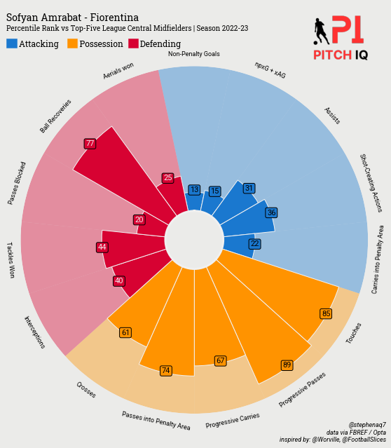
This code defines a function, create_single_Pizza, which generates a radar chart (pizza plot) visualizing various performance metrics for a given football player. Here are the steps:
1: Define Parameters: Specify a list of performance metrics (params) that will be visualized on the pizza plot.
2: Retrieve Player Data: Query the main player database (EU_TOP_5_DB) for the subset of data related to the specified player.
3: Generate Advanced Data: Extract advanced statistical data for the player using their scouting report links. Organize the data into two DataFrames - one for per-90 statistics and another for percentiles.
4: Prepare Data for Visualization: Convert necessary columns to numeric, extract values, and obtain additional information about the player’s team.
5: Set Up Pizza Plot: Set up the parameters for the pizza plot, such as colors, styles, and layout.
6: Create Pizza Plot: Use the mplsoccer library to create a radar chart (pizza plot) with slices representing different performance metrics.
7: Add Title and Credits: Include a title, subtitle, and credits on the plot to provide context and acknowledgment.
8: Save and Display: Save the generated pizza plot as an image file and display it.
Note: This function visualizes a player’s performance in attacking, possession, and defending based on the specified metrics. The resulting pizza plot provides an intuitive overview of the player’s strengths and weaknesses in various aspects of the game.
def create_single_Pizza(player_name):
    # parameter list
    params = [
        "Non-Penalty Goals", "npxG + xAG", "Assists",
        "Shot-Creating Actions", "Carries into Penalty Area",
        "Touches", "Progressive Passes", "Progressive Carries",
        "Passes into Penalty Area", "Crosses",
        "Interceptions", "Tackles Won",
        "Passes Blocked", "Ball Recoveries", "Aerials won"
    ]

    subset_of_data = EU_TOP_5_DB.query('Player == @player_name' )
    scout_links = list(subset_of_data.scouting_url.unique())
    appended_data_percentile = generate_advanced_data(scout_links)[1]
    appended_data_percentile = appended_data_percentile[params]
    cols = appended_data_percentile.columns
    appended_data_percentile[cols] = appended_data_percentile[cols].apply(pd.to_numeric)
    params = list(appended_data_percentile.columns)
    # params = params[1:]


    values = appended_data_percentile.iloc[0].values.tolist()
    # values = values[1:]

    get_clubs = subset_of_data[subset_of_data.Player.isin([player_name])]
    link_list = list(get_clubs.urls.unique())
    title_vars = []
    for x in link_list:
        warnings.filterwarnings("ignore")
        html_content = requests.get(x).text.replace('<!--', '').replace('-->', '')
        df2 = pd.read_html(html_content)
        df2[5].columns = df2[5].columns.droplevel(0)
        stats2 = df2[5]
        key_vars = stats2[["Season","Age","Squad"]]
        key_vars = key_vars[key_vars.Season.isin(["2021-2022"])]
        title_vars.append(key_vars)
    title_vars = pd.concat(title_vars)
    teams = list(title_vars.Squad.unique())[0]


    style.use('fivethirtyeight')


    # color for the slices and text
    slice_colors = ["#1A78CF"] * 5 + ["#FF9300"] * 5 + ["#D70232"] * 5
    text_colors = ["#000000"] * 10 + ["#F2F2F2"] * 5

    # instantiate PyPizza class
    baker = PyPizza(
        params=params,                  # list of parameters
        background_color="#EBEBE9",     # background color
        straight_line_color="#EBEBE9",  # color for straight lines
        straight_line_lw=1,             # linewidth for straight lines
        last_circle_lw=0,               # linewidth of last circle
        other_circle_lw=0,              # linewidth for other circles
        inner_circle_size=20            # size of inner circle
    )

    # plot pizza
    fig, ax = baker.make_pizza(
        values,                          # list of values
        figsize=(8, 8.5),                # adjust figsize according to your need
        color_blank_space="same",        # use same color to fill blank space
        slice_colors=slice_colors,       # color for individual slices
        value_colors=text_colors,        # color for the value-text
        value_bck_colors=slice_colors,   # color for the blank spaces
        blank_alpha=0.4,                 # alpha for blank-space colors
        kwargs_slices=dict(
            edgecolor="#F2F2F2", zorder=2, linewidth=1
        ),                               # values to be used when plotting slices
        kwargs_params=dict(
            color="#000000", fontsize=9,
            fontproperties=font_normal.prop, va="center"
        ),                               # values to be used when adding parameter
        kwargs_values=dict(
            color="#000000", fontsize=11,
            fontproperties=font_normal.prop, zorder=3,
            bbox=dict(
                edgecolor="#000000", facecolor="cornflowerblue",
                boxstyle="round,pad=0.2", lw=1
            )
        )                                # values to be used when adding parameter-values
    )

    # add title
    fig.text(
        0.05, 0.985, f"{player_name} - {teams}", size=14,
        ha="left", fontproperties=font_bold.prop, color="#000000"
    )

    # add subtitle
    fig.text(
        0.05, 0.963,
        f"Percentile Rank vs Top-Five League {subset_of_data.position_group.unique()[0]} | Season 2022-23",
        size=10,
        ha="left", fontproperties=font_bold.prop, color="#000000"
    )

    # add credits
    CREDIT_1 = "@stephenaq7\ndata via FBREF / Opta"
    CREDIT_2 = "inspired by: @Worville, @FootballSlices"

    fig.text(
        0.99, 0.005, f"{CREDIT_1}\n{CREDIT_2}", size=9,
        fontproperties=font_italic.prop, color="#000000",
        ha="right"
    )

    # add text
    fig.text(
        0.08, 0.925, "Attacking          Possession        Defending", size=12,
        fontproperties=font_bold.prop, color="#000000"
    )

    # add rectangles
    fig.patches.extend([
        plt.Rectangle(
            (0.05, 0.9225), 0.025, 0.021, fill=True, color="#1a78cf",
            transform=fig.transFigure, figure=fig
        ),
        plt.Rectangle(
            (0.2, 0.9225), 0.025, 0.021, fill=True, color="#ff9300",
            transform=fig.transFigure, figure=fig
        ),
        plt.Rectangle(
            (0.351, 0.9225), 0.025, 0.021, fill=True, color="#d70232",
            transform=fig.transFigure, figure=fig
        ),
    ])

    # add image
    ### Add Stats by Steve logo
    ax3 = fig.add_axes([0.80, 0.075, 0.15, 1.75])
    ax3.axis('off')
    img = image.imread('/Users/stephenahiabah/Desktop/GitHub/Webs-scarping-for-Fooball-Data-/outputs/piqmain.png')
    ax3.imshow(img)
    plt.savefig(
	f"Twitter_img/{player_name} - plot.png",
	dpi = 500,
	facecolor = "#EFE9E6",
	bbox_inches="tight",
    edgecolor="none",
	transparent = False
)
    plt.show()
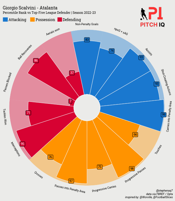
As an Arsenal fan, our defensive collapse two seasons running gives me sleepness nights, so I’m always on the lookout for promising centre back. One player I really like is Giorgio Scalvini, so lets use him as an example for this analysis
players = ['Giorgio Scalvini']
for player in players:
    create_single_Pizza(player)
This simple loop generates a pizza plot for a single football player, in this case, Giorgio Scalvini, resulting in the following visual:
Creation of Comparison Pizza Chart
Here’s an explanation of the create_comparison_pizza code:
1: Define Parameters: The function begins by defining a list of parameters representing various performance metrics for the pizza plot.
2: Generate Values for Player 1: The function uses the generate_values function to obtain performance values and team information for the first player based on the specified parameters.
3: Generate Values for Player 2: Similar to Player 1, the function obtains performance values and team information for the second player using the generate_values function.
4: Set Up PyPizza Class: The PyPizza class is configured with specific styling, including color ranges and offsets, to prepare for creating the pizza plot.
5: Create Pizza Plot: The pizza plot is generated using the PyPizza class, incorporating values for both players to compare their performance. Colors, sizes, and other plot settings are adjusted accordingly.
6: Adjust Texts and Add Title: Texts on the pizza plot are adjusted for better readability, and a title is added to indicate the comparison between the two players.
7: Add Credits and Image: Credits and additional information are included at the bottom of the plot, acknowledging the data source and providing additional details. An image is also added to the plot.
8: Save and Display Plot: The final pizza plot is saved as an image file, and the plt.show() function is used to display the plot.
This function essentially creates a visual representation (pizza plot) comparing the performance of two football players based on specified performance metrics.
def create_comparison_pizza(player1_name, player2_name):

    params = [
        "Non-Penalty Goals", "npxG + xAG", "Assists",
        "Shot-Creating Actions", "Carries into Penalty Area",
        "Touches", "Progressive Passes", "Progressive Carries",
        "Passes into Penalty Area", "Crosses",
        "Interceptions", "Tackles Won",
        "Passes Blocked", "Ball Recoveries", "Aerials won"
    ]

    def generate_values(player_name,params):
        subset_of_data = EU_TOP_5_DB.query('Player == @player_name')
        scout_links = list(subset_of_data.scouting_url.unique())
        appended_data_percentile = generate_advanced_data(scout_links)[0]
        appended_data_percentile = appended_data_percentile[params]
        cols = appended_data_percentile.columns
        appended_data_percentile[cols] = appended_data_percentile[cols].apply(pd.to_numeric)
        params = list(appended_data_percentile.columns)

        values = appended_data_percentile.iloc[0].values.tolist()

        get_clubs = subset_of_data[subset_of_data.Player.isin([player_name])]
        link_list = list(get_clubs.urls.unique())
        title_vars = []
        for x in link_list:
            warnings.filterwarnings("ignore")
            html_content = requests.get(x).text.replace('<!--', '').replace('-->', '')
            df2 = pd.read_html(html_content)
            df2[5].columns = df2[5].columns.droplevel(0)
            stats2 = df2[5]
            key_vars = stats2[["Season", "Age", "Squad"]]
            key_vars = key_vars[key_vars.Season.isin(["2021-2022"])]
            title_vars.append(key_vars)
        title_vars = pd.concat(title_vars)
        teams = list(title_vars.Squad.unique())[0]

        return values, teams


    values, teams_1 = generate_values(player1_name, params)
    values_2, teams_2 = generate_values(player2_name,params)


    style.use('fivethirtyeight')


    min_range = [min(value, value_2) * 0.5 for value, value_2 in zip(values, values_2)]
    max_range = [max(value, value_2) * 1.05 for value, value_2 in zip(values, values_2)]


    # pass True in that parameter-index whose values are to be adjusted
    # here True values are passed for "Pressure Regains", "pAdj Tackles" params
    params_offset = [True] * len(max_range)

    # instantiate PyPizza class
    baker = PyPizza(
        params=params,
        min_range=min_range,        # min range values
        max_range=max_range,        # max range values
        background_color="#222222", straight_line_color="#000000",
        last_circle_color="#000000", last_circle_lw=2.5, other_circle_lw=0,
        other_circle_color="#000000", straight_line_lw=1
    )

    # plot pizza
    fig, ax = baker.make_pizza(
        values,                     # list of values
        compare_values=values_2,    # passing comparison values
        figsize=(10, 10),             # adjust figsize according to your need
        color_blank_space="same",   # use same color to fill blank space
        blank_alpha=0.4,            # alpha for blank-space colors
        param_location=110,         # where the parameters will be added
        kwargs_slices=dict(
            facecolor="#1A78CF", edgecolor="#000000",
            zorder=1, linewidth=1
        ),                          # values to be used when plotting slices
        kwargs_compare=dict(
            facecolor="#ff9300", edgecolor="#222222", zorder=3, linewidth=1,
        ),                          # values to be used when plotting comparison slices
        kwargs_params=dict(
            color="#F2F2F2", fontsize=12, zorder=5,
            fontproperties=font_normal.prop, va="center"
        ),                          # values to be used when adding parameter
        kwargs_values=dict(
            color="#000000", fontsize=12,
            fontproperties=font_normal.prop, zorder=3,
            bbox=dict(
                edgecolor="#000000", facecolor="#1A78CF",
                boxstyle="round,pad=0.2", lw=1
            )
        ),                           # values to be used when adding parameter-values
        kwargs_compare_values=dict(
            color="#000000", fontsize=12,
            fontproperties=font_normal.prop, zorder=3,
            bbox=dict(
                edgecolor="#000000", facecolor="#FF9300",
                boxstyle="round,pad=0.2", lw=1
            )
        )                            # values to be used when adding comparison-values
    )


    # adjust the texts
    # to adjust text for comparison-values-text pass adj_comp_values=True
    baker.adjust_texts(params_offset, offset=-0.17)

    # add title
    fig_text(
        0.515, 0.99, f"<{player1_name}> vs <{player2_name}>",
        size=16, fig=fig,
        highlight_textprops=[{"color": '#1A78CF'}, {"color": '#FF9300'}],
        ha="center", fontproperties=font_bold.prop, color="#F2F2F2"
    )
    # add credits
    CREDIT_1 = "@stephenaq7\ndata via FBREF / Opta"
    CREDIT_2 = "inspired by: @Worville, @FootballSlices"

    fig.text(
        0.99, 0.005, f"{CREDIT_1}\n{CREDIT_2}", size=9,
        fontproperties=font_italic.prop, color="#F2F2F2",
        ha="right"
    )

    # add image
    ### Add Stats by Steve logo
    ax3 = fig.add_axes([0.80, 0.075, 0.15, 1.75])
    ax3.axis('off')
    img = image.imread('/Users/stephenahiabah/Desktop/GitHub/Webs-scarping-for-Fooball-Data-/outputs/PITCH IQ PRIMARY.png')
    ax3.imshow(img)
    plt.savefig(
    f"Twitter_img/{player1_name}> vs <{player2_name} - plot.png",
    dpi = 500,
    facecolor = "#EFE9E6",
    bbox_inches="tight",
    edgecolor="none",
    transparent = False
    )

    plt.show()
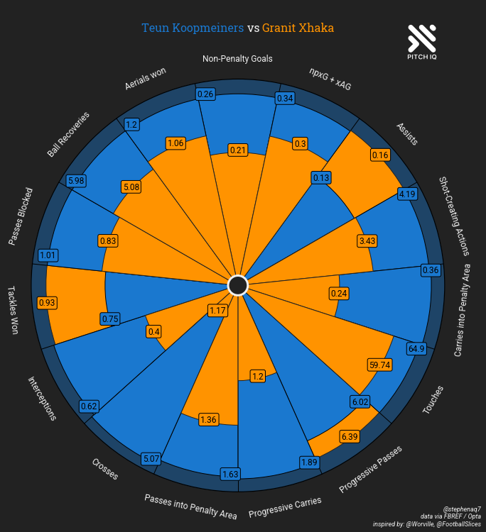
In this comparison, staying with the Atalanta theme, I’ve decided to pick Teun Koopmeiners, who I think in the eye test looks quite similar to Granit Xhaka, so lets put that to the test.
create_comparison_pizza('Teun Koopmeiners', 'Granit Xhaka')
Conclusion
In conclusion, this post serves as a valuable addition to a series of tutorials aimed at empowering users to craft dynamic and replicable functions for generating insightful data visualizations, especially tailored for social media or personal enjoyment. In the next iteration I’ll be going over radar charts. I hope you found this useful.
Thanks for reading
Steve

Comments